The Confusion is Real: GRAPHIC -- A Network Science Approach to Confusion Matrices in Deep Learning
Pith reviewed 2026-05-15 20:15 UTC · model grok-4.3
The pith
Confusion matrices from intermediate layers can be turned into directed graphs to track how neural networks learn class relationships over training.
A machine-rendered reading of the paper's core claim, the machinery that carries it, and where it could break.
Core claim
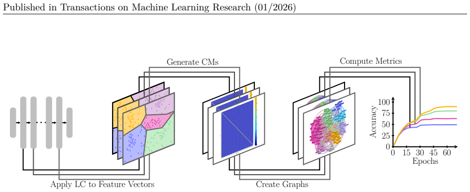
GRAPHIC converts confusion matrices derived from linear classifiers on intermediate-layer activations into adjacency matrices of directed graphs and then applies network-science tools to measure and display the evolution of class relationships throughout training, thereby exposing patterns of linear separability, dataset ambiguities, and architectural differences.
What carries the argument
Directed graphs whose edges are weighted by confusion-matrix entries from linear probes on successive layers, with standard network metrics used to track changes across training.
If this is right
- Linear separability of classes can be monitored layer by layer and epoch by epoch.
- Labeling ambiguities in a dataset become visible as persistent high-confusion edges in the graph.
- Specific inter-class similarities that hinder performance, such as flatfish and man, are identified automatically.
- Different network architectures produce distinguishable patterns in the evolution of their class graphs.
- Human studies can be used to validate whether the detected confusions reflect genuine data issues.
Where Pith is reading between the lines
- The same graph-construction step could be applied to sequence models to expose confusion patterns among tokens or actions.
- Early identification of high-confusion subgraphs might guide data-augmentation or curriculum strategies.
- Comparing class graphs across datasets could quantify how data distribution shapes what a model treats as similar.
- The method offers a possible bridge between model-internal representations and human perceptual categories when the human study matches the graph findings.
Load-bearing premise
Confusion matrices produced by linear classifiers on intermediate activations capture the class relationships that matter for the full nonlinear model's decisions.
What would settle it
If the graph-derived metrics fail to correlate with observed misclassification rates or with human judgments of class similarity on an independent dataset, the approach would not deliver the claimed insights.
Figures


read the original abstract
Explainable artificial intelligence has emerged as a promising field of research to address reliability concerns in artificial intelligence. Despite significant progress in explainable artificial intelligence, few methods provide a systematic way to visualize and understand how classes are confused and how their relationships evolve as training progresses. In this work, we present GRAPHIC, an architecture-agnostic approach that analyzes neural networks on a class level. It leverages confusion matrices derived from intermediate layers using linear classifiers. We interpret these as adjacency matrices of directed graphs, allowing tools from network science to visualize and quantify learning dynamics across training epochs and intermediate layers. GRAPHIC provides insights into linear class separability, dataset issues, and architectural behavior, revealing, for example, similarities between flatfish and man and labeling ambiguities validated in a human study. In summary, by uncovering real confusions, GRAPHIC offers new perspectives on how neural networks learn. The code is available at https://github.com/Johanna-S-Froehlich/GRAPHIC.
Editorial analysis
A structured set of objections, weighed in public.
Referee Report
Summary. The paper introduces GRAPHIC, an architecture-agnostic method that derives confusion matrices by training linear classifiers on intermediate-layer activations of a neural network, interprets these matrices as adjacency matrices of directed graphs, and applies standard network-science metrics (centrality, community detection, dynamics across epochs) to analyze class relationships and learning progress. It presents qualitative examples of discovered class similarities (e.g., flatfish and man) and reports a human validation study confirming labeling ambiguities.
Significance. If the linear-probe matrices can be shown to faithfully reflect the full model's class confusions, the approach would supply a systematic, visualizable way to track how class separability evolves during training and to flag dataset or architectural issues. The human-study component adds modest credibility to the labeling-ambiguity claim. At present the significance remains limited because the core proxy has not been validated against the model's actual output confusion matrix, leaving open whether the network metrics yield insights beyond conventional confusion-matrix inspection.
major comments (2)
- [Methods (linear-probe construction)] The construction of confusion matrices via linear probes on intermediate activations (described in the Methods section) is not accompanied by any direct quantitative comparison to the confusion matrix produced by the full end-to-end model. Because later layers apply non-linear transformations, the linear decision boundaries at layer l need not reproduce the model's actual output confusions; all downstream network-science claims therefore rest on an unverified proxy.
- [Experiments and Results] The experimental evaluation (qualitative examples plus human study) provides no quantitative metrics, ablation studies, or statistical controls that would demonstrate the robustness or added value of the network-science metrics over standard confusion-matrix analysis. This absence makes it impossible to assess whether the reported insights are reproducible or merely post-hoc interpretations.
minor comments (1)
- [Abstract / Introduction] The abstract and introduction repeatedly use the phrase 'real confusions' without a precise definition; a short clarifying sentence would help readers distinguish the probe-derived matrices from the model's output matrix.
Simulated Author's Rebuttal
We thank the referee for the constructive comments, which identify key areas where additional validation and quantification can strengthen the manuscript. We address each major comment below and will incorporate revisions to provide the requested comparisons and metrics.
read point-by-point responses
-
Referee: [Methods (linear-probe construction)] The construction of confusion matrices via linear probes on intermediate activations (described in the Methods section) is not accompanied by any direct quantitative comparison to the confusion matrix produced by the full end-to-end model. Because later layers apply non-linear transformations, the linear decision boundaries at layer l need not reproduce the model's actual output confusions; all downstream network-science claims therefore rest on an unverified proxy.
Authors: We agree that a direct quantitative validation of the linear-probe proxy against the full model's output confusion matrix is a valuable addition. Although the probes are designed to isolate linear class separability at each layer (a complementary perspective to the end-to-end non-linear boundaries), we will add a new subsection in the Methods and Results that computes the final-layer probe confusion matrix and compares it to the model's actual test-set confusion matrix. The comparison will report agreement percentage, normalized Frobenius distance, and element-wise Pearson correlation to quantify fidelity. This will be included in the revised manuscript. revision: yes
-
Referee: [Experiments and Results] The experimental evaluation (qualitative examples plus human study) provides no quantitative metrics, ablation studies, or statistical controls that would demonstrate the robustness or added value of the network-science metrics over standard confusion-matrix analysis. This absence makes it impossible to assess whether the reported insights are reproducible or merely post-hoc interpretations.
Authors: We acknowledge the absence of quantitative evaluation and agree that it limits assessment of added value. In the revision we will augment the Experiments section with: (i) quantitative tracking of network metrics (e.g., betweenness centrality, modularity) across epochs with statistical significance tests; (ii) an ablation comparing class-similarity rankings derived from GRAPHIC versus direct confusion-matrix inspection; and (iii) inter-rater agreement statistics (Fleiss' kappa) and confidence intervals for the human validation study. These additions will demonstrate reproducibility and the incremental insight provided by the network-science tools. revision: yes
Circularity Check
No circularity: purely descriptive application of standard network metrics to derived confusion matrices
full rationale
The paper constructs confusion matrices via linear probes on intermediate-layer activations, interprets them as directed graphs, and applies off-the-shelf network-science metrics (centrality, community detection, dynamics across epochs). No parameters are fitted to a subset and then re-used as a 'prediction'; no equations reduce by construction to the inputs; no load-bearing self-citations or uniqueness theorems are invoked. The method is self-contained as an analysis pipeline whose outputs are direct computations on the proxy matrices, not tautological re-labelings or re-derivations of the same quantities.
Axiom & Free-Parameter Ledger
axioms (2)
- domain assumption Confusion matrices derived from linear classifiers on intermediate activations represent meaningful class relationships inside the network
- domain assumption Network-science metrics applied to these graphs yield interpretable and actionable insights into learning dynamics
Lean theorems connected to this paper
-
IndisputableMonolith/Foundation/RealityFromDistinction.leanreality_from_one_distinction unclear?
unclearRelation between the paper passage and the cited Recognition theorem.
We employ the method introduced by Dugué & Perez (2015) to identify community structures... modularity Q
What do these tags mean?
- matches
- The paper's claim is directly supported by a theorem in the formal canon.
- supports
- The theorem supports part of the paper's argument, but the paper may add assumptions or extra steps.
- extends
- The paper goes beyond the formal theorem; the theorem is a base layer rather than the whole result.
- uses
- The paper appears to rely on the theorem as machinery.
- contradicts
- The paper's claim conflicts with a theorem or certificate in the canon.
- unclear
- Pith found a possible connection, but the passage is too broad, indirect, or ambiguous to say the theorem truly supports the claim.
Reference graph
Works this paper leans on
-
[1]
Understanding intermediate layers using linear classifier probes
Guillaume Alain and Yoshua Bengio. Understanding intermediate layers using linear classifier probes.arXiv preprint arXiv:1610.01644,
work page internal anchor Pith review Pith/arXiv arXiv
-
[2]
Brundage, Min Wu, and Sanghamitra Dutta
Pranjal Atrey, Michael P. Brundage, Min Wu, and Sanghamitra Dutta. Demystifying the accuracy- interpretability trade-off: A case study of inferring ratings from reviews.arXiv preprint arXiv:2503.07914,
-
[3]
Jan Niklas Böhm, Philipp Berens, and Dmitry Kobak
doi: 10.1109/TVCG.2017.2744683. Jan Niklas Böhm, Philipp Berens, and Dmitry Kobak. Unsupervised visualization of image datasets using contrastive learning. InInternational Conference on Learning Representations
-
[4]
org/de/worterbuch/englisch/tabby
URLhttps://dictionary.cambridge. org/de/worterbuch/englisch/tabby. 13 Published in Transactions on Machine Learning Research (01/2026) David M Chan, Roshan Rao, Forrest Huang, and John F Canny. t-SNE-CUDA: GPU-accelerated t-SNE and its applications to modern data. InProceedings of the 30th International Symposium on Computer Architecture and High Performa...
work page 2026
-
[5]
Distilling the Knowledge in a Neural Network
Geoffrey Hinton, Oriol Vinyals, and Jeff Dean. Distilling the knowledge in a neural network.arXiv preprint arXiv:1503.02531,
work page internal anchor Pith review Pith/arXiv arXiv
-
[6]
Confusion graph: Detecting confusion communities in large scale image classification
Ruochun Jin, Yong Dou, Yueqing Wang, and Xin Niu. Confusion graph: Detecting confusion communities in large scale image classification. In Proceedings of the International Joint Conference on Artificial Intelligence, pp. 1980–1986,
work page 1980
-
[7]
Hamid Karimi, Tyler Derr, and Jiliang Tang. Characterizing the decision boundary of deep neural networks. arXiv preprint arXiv:1912.11460,
-
[8]
14 Published in Transactions on Machine Learning Research (01/2026) Pang Wei Koh, Thao Nguyen, Yew Siang Tang, Stephen Mussmann, Emma Pierson, Been Kim, and Percy Liang. Concept bottleneck models. In Hal Daumé III and Aarti Singh (eds.),International Conference on Machine Learning, volume 119 ofProceedings of Machine Learning Research, pp. 5338–5348. PMLR...
work page 2026
-
[9]
Fuseini Mumuni and Alhassan Mumuni. Explainable artificial intelligence (xai): From inherent explainability to large language models.arXiv preprint arXiv:2501.09967,
-
[10]
org/docs/stable/generated/torch.optim.lr_scheduler.ReduceLROnPlateau.html
URL https://docs.pytorch. org/docs/stable/generated/torch.optim.lr_scheduler.ReduceLROnPlateau.html. 15 Published in Transactions on Machine Learning Research (01/2026) Maithra Raghu, Thomas Unterthiner, Simon Kornblith, Chiyuan Zhang, and Alexey Dosovitskiy. Do vision transformers see like convolutional neural networks?Advances in Neural Information Proc...
work page 2026
-
[11]
Cuevas-Tello, Jose Nunez-Varela, Cesar Puente, and Alejandra G
Gabriela Rangel, Juan C. Cuevas-Tello, Jose Nunez-Varela, Cesar Puente, and Alejandra G. Silva-Trujillo. A survey on convolutional neural networks and their performance limitations in image recognition tasks. Journal of Sensors, 2024(1):2797320,
work page 2024
-
[12]
Train- ing a vision transformer from scratch in less than 24 hours with 1 gpu
Saghar Irandoust, Thibaut Durand, Yunduz Rakhmangulova, Wenjie Zi, and Hossein Hajimirsadeghi. Train- ing a vision transformer from scratch in less than 24 hours with 1 gpu. InHas it Trained Yet? NeurIPS 2022 Workshop,
work page 2022
-
[13]
arXiv preprint arXiv:2402.01761 , year=
Chandan Singh, Jeevana Priya Inala, Michel Galley, Rich Caruana, and Jianfeng Gao. Rethinking inter- pretability in the era of large language models.arXiv preprint arXiv:2402.01761,
-
[14]
Post-hoc concept bottleneck models
16 Published in Transactions on Machine Learning Research (01/2026) Mert Yuksekgonul, Maggie Wang, and James Zou. Post-hoc concept bottleneck models. InInternational Conference on Learning Representations,
work page 2026
-
[15]
This requires a dataset, where concept annotations must be available during training
are intrinsically interpretable architectures that explicitly decompose prediction into two stages: predicting human-defined concepts and then using these concepts to predict the final class. This requires a dataset, where concept annotations must be available during training. Post-hoc concept bottleneck models have also been proposed (Yuksekgonul et al.,...
work page 2023
-
[16]
visualize representations by first com- puting pairwise similarities between samples and then mapping them into a low-dimensional space. When 17 Published in Transactions on Machine Learning Research (01/2026) these similarities are computed in the input space, however, it is not guaranteed that distance measures such as the Euclidean distance in high-dim...
work page 2026
-
[17]
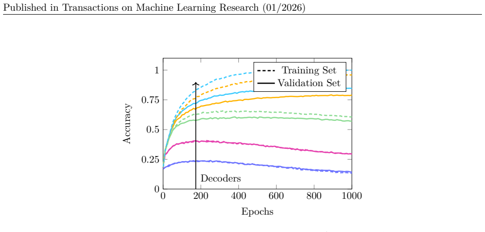
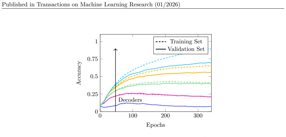
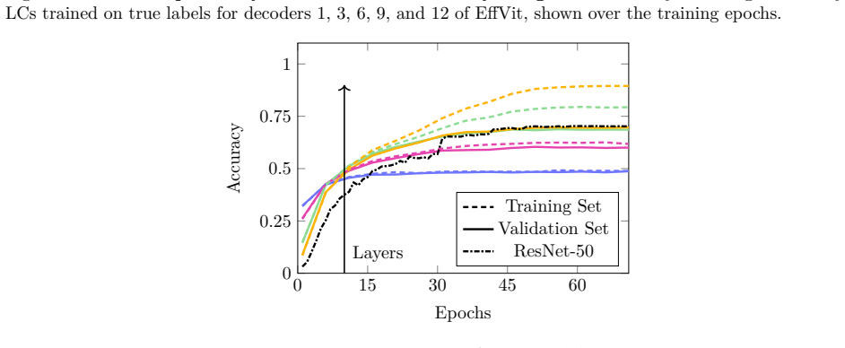
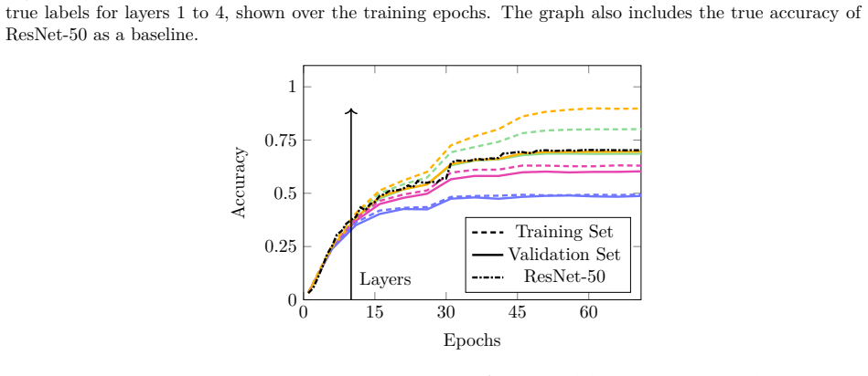
It shows the accuracy of the different layers of ResNet-50 determined by LCs trained on the true labels in comparison to the true accuracy of ResNet-50. Here we see an increase ending in a stagnation, rather than a drop. 18 Published in Transactions on Machine Learning Research (01/2026) 0 200 400 600 800 10000 0.25 0.5 0.75 1 Decoders Epochs Accuracy Tra...
work page 2026
-
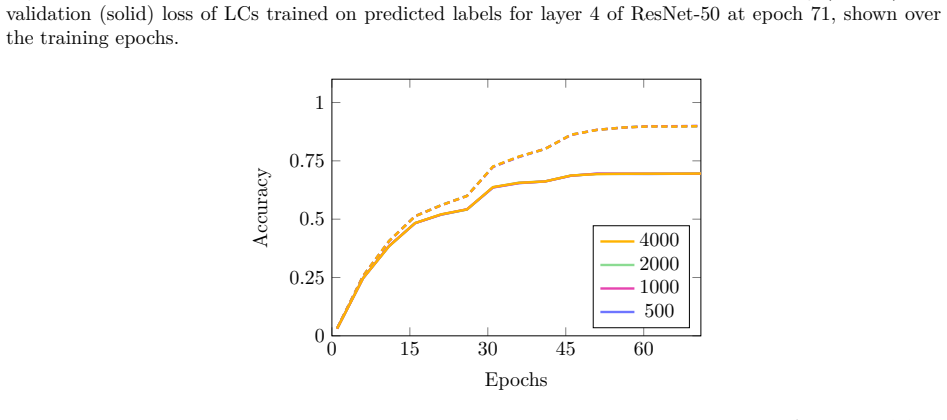
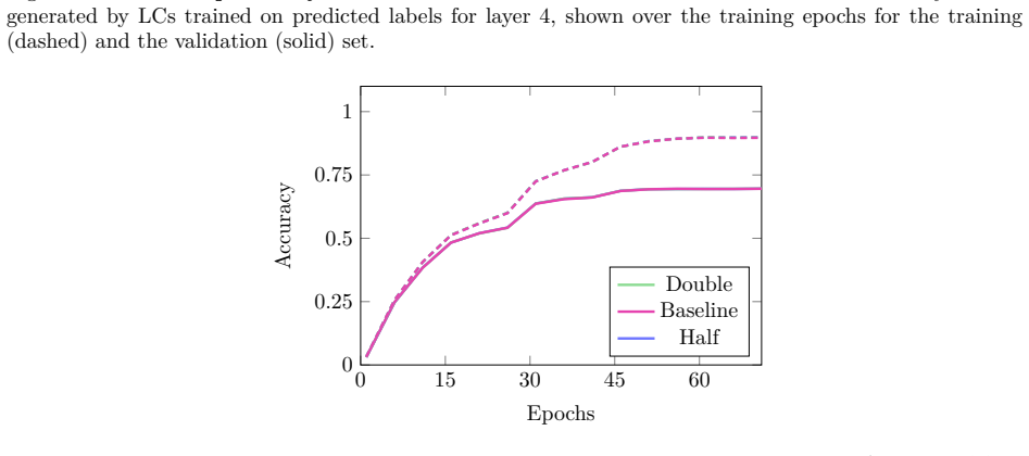
[18]
As discussed in Appendix A.6 our results are robust to the LC training and this is confirmed here again. 22 Published in Transactions on Machine Learning Research (01/2026) 0 15 30 45 600 0.25 0.5 0.75 1 Layers Epochs Modularity Baseline Regularization Figure 17: Layer-wise modularity over training epochs for ResNet-50 with and without regu- larization. M...
work page 2026
-
[19]
Even though the number of nodes remains unchanged, the reduced edge set leads to fewer overlapping structures. This can be especially helpful in the early stages of training as there are more confusions overall. To address larger numbers of classes, a second approach is to inspect individual CCs instead of the full graph. The strongest confusions typicall...
work page 2026
-
[20]
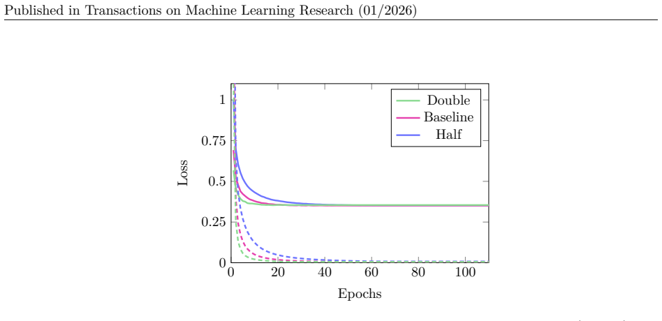
The modularity for layer 4 on the training set tracks the accuracy (cf
show an interesting trend. The modularity for layer 4 on the training set tracks the accuracy (cf. Figure 11), with similar steps. The steps stem from the used scheduler ReduceLROnPlateau (PyTorch Foundation, 2025), which reduces the learning rate if the loss stagnates. For both the predicted labels and the true labels (cf. Figure 31), the grouping streng...
work page 2025
-
[21]
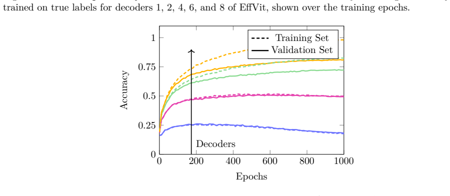
Because EffVit is trained for only 24 hours rather than to full convergence, the increase in modularity is small as the number of confusions is still relatively high. 30 Published in Transactions on Machine Learning Research (01/2026) 0 15 30 45 600 0.25 0.5 0.75 1 Layers Epochs Modularity Training Set Validation Set Figure 31:Layer-wise modularity over t...
work page 2026
-
[22]
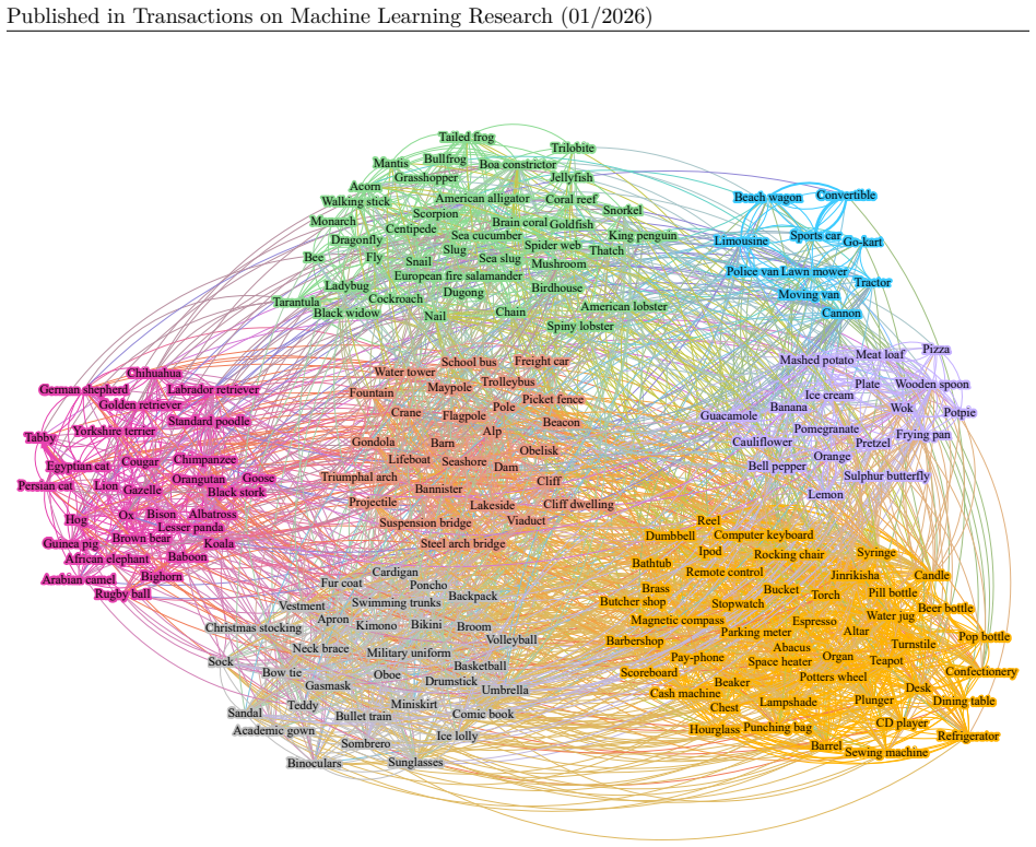
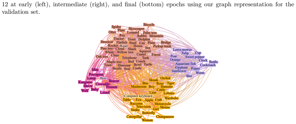
It depicts the human CC of layer 2 of the converged ResNet-50 model. 33 Published in Transactions on Machine Learning Research (01/2026) Apple Aquarium fish Bicycle Chair Computer keyboard Orange Pear Poppy Sea Snake Sweet pepper Telephone Crocodile Elephant Possum Shark Baby Turtle Bear Beaver Kangaroo Skyscraper Bed Bee Mushroom Beetle Cup Bottle Bowl B...
work page 2026
-
[23]
It increases slightly for layer three and four for the later training epochs
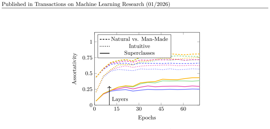
The assortativity is similar for all layers and around 0.3. It increases slightly for layer three and four for the later training epochs. This still suggests a group structure, though it is much less distinct than with the correct group assignments. Since we are working with only two classes, many individual categories – whether labeled as man-made or nat...
work page 2026
-
[24]
For the image of the boy the accuracy for the first image is 42%, the duplicate is identified with 61% accuracy. For the image of the girl the initial labeling accuracy is 39%, the duplicate is labeled correctly with an accuracy of 23%. 71% of the participants changed their mind about their initial 41 Published in Transactions on Machine Learning Research...
work page 2026
discussion (0)
Sign in with ORCID, Apple, or X to comment. Anyone can read and Pith papers without signing in.