Causal Spatio-Temporal Sound Field Reconstruction
Pith reviewed 2026-05-21 06:55 UTC · model grok-4.3
The pith
A causal spatio-temporal LMMSE estimator reconstructs sound fields more accurately from short causal measurement windows by deriving a covariance from the wave equation solution under stationary stochastic sources.
A machine-rendered reading of the paper's core claim, the machinery that carries it, and where it could break.
Core claim
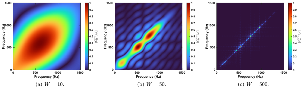
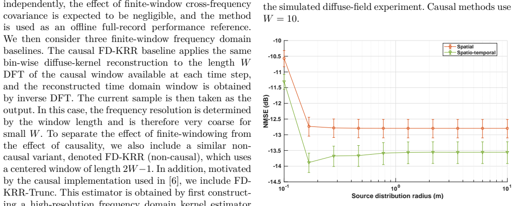
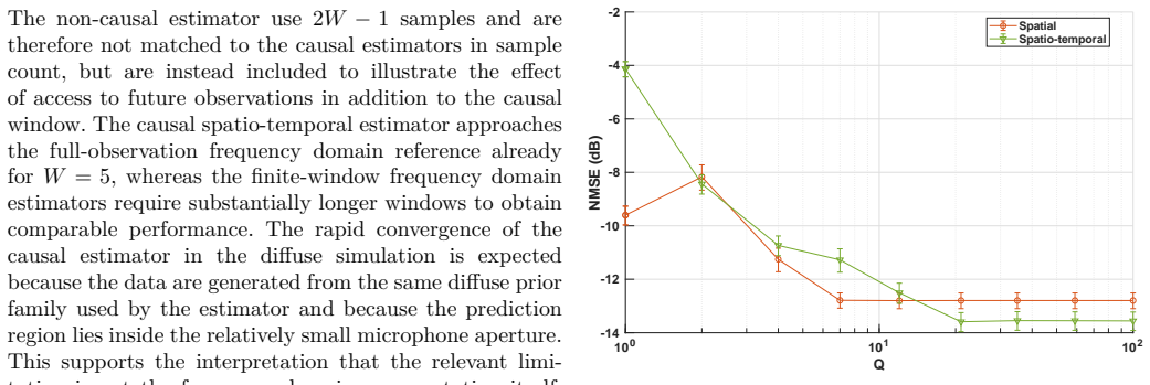
We formulate a causal finite-window spatio-temporal linear minimum mean-square error estimator for sound field reconstruction. The sound field is modeled as the solution to the wave equation driven by a stationary stochastic spatio-temporal source distribution, which induces a physically interpretable covariance function. It is shown that this covariance function is closely related to the classical diffuse-field coherence model. Since the computational complexity grows rapidly with the number of spatio-temporal observations, we formulate a budget-constrained spatio-temporal sample selection approach to minimize the posterior reconstruction variance. The proposed estimator and sampling method
What carries the argument
The covariance function induced by modeling the sound field as the solution to the wave equation driven by a stationary stochastic spatio-temporal source distribution, which is inserted into the causal finite-window spatio-temporal linear minimum mean-square error estimator.
If this is right
- The estimator outperforms frequency-domain finite-window baselines in short-window reconstruction on both simulated and measured data.
- The derived covariance function is closely related to the classical diffuse-field coherence model.
- A budget-constrained spatio-temporal sample selection approach minimizes posterior reconstruction variance under computational limits.
- The overall approach remains effective when applied to real measured sound fields.
Where Pith is reading between the lines
- The same wave-equation-plus-stationary-source modeling step could be reused for causal reconstruction of other linear wave fields such as electromagnetic or seismic waves.
- Relaxing the stationarity assumption on the driving source distribution would be a natural next step for handling time-varying acoustic environments.
- The sample-selection strategy might generalize to adaptive placement of microphones in real-time sensing arrays.
- Lower-latency accurate field estimates could directly benefit closed-loop active noise control or immersive audio rendering systems.
Load-bearing premise
The sound field can be accurately represented as the solution to the wave equation driven by a stationary stochastic spatio-temporal source distribution that induces the covariance used in the estimator.
What would settle it
Direct side-by-side tests on measured causal microphone data that show the proposed estimator yields no lower reconstruction error than standard frequency-domain finite-window methods for short windows would refute the claimed improvement.
Figures


read the original abstract
In sound field control applications, it is commonly assumed that one has access to an accurate representation of the sound field in the region of interest. This is a problematic assumption since the reconstruction of a sound field from available microphone measurements is especially challenging in real-time applications where only causal measurements are available. Notably, causal time-windowed observations introduce correlation between frequency components, making sound field reconstruction methods that process each frequency band independently sub-optimal. In this work, we formulate a causal finite-window spatio-temporal linear minimum mean-square error estimator for sound field reconstruction. The sound field is modeled as the solution to the wave equation driven by a stationary stochastic spatio-temporal source distribution, which induces a physically interpretable covariance function. It is shown that this covariance function is closely related to the classical diffuse-field coherence model. Since the computational complexity grows rapidly with the number of spatio-temporal observations, we formulate a budget-constrained spatio-temporal sample selection approach to minimize the posterior reconstruction variance. The proposed estimator and sampling strategy are evaluated using both simulated and measured sound fields, demonstrating improved short-window reconstruction compared to frequency domain finite-window baselines.
Editorial analysis
A structured set of objections, weighed in public.
Referee Report
Summary. The manuscript formulates a causal finite-window spatio-temporal linear minimum mean-square error (LMMSE) estimator for sound field reconstruction from microphone measurements. The sound field is modeled as the solution to the wave equation driven by a stationary stochastic spatio-temporal source distribution, inducing a physically interpretable covariance function closely related to the classical diffuse-field coherence model. A budget-constrained spatio-temporal sample selection strategy is introduced to minimize posterior reconstruction variance. The estimator and sampling approach are evaluated on both simulated and measured sound fields, demonstrating improved short-window reconstruction performance relative to frequency-domain finite-window baselines.
Significance. If the central claims hold under the stated modeling assumptions, the work offers a principled extension of LMMSE estimation to causal spatio-temporal settings in acoustics. The derivation of the covariance directly from the wave equation provides a physically grounded alternative to purely empirical or frequency-independent models, which could benefit real-time applications such as sound field control and virtual acoustics by capturing cross-frequency correlations induced by finite causal windows.
major comments (2)
- [Abstract and modeling section] Abstract and modeling section: The stationarity assumption on the driving stochastic spatio-temporal source distribution is load-bearing for the optimality of the causal finite-window LMMSE estimator and the claimed superiority over frequency-domain baselines. The induced covariance is derived under this premise, yet the manuscript does not appear to test robustness when the assumption is violated (as is common for speech, music, or transient signals). A concrete sensitivity analysis or comparison on non-stationary data would be required to substantiate the short-window gains.
- [Evaluation section] Evaluation section: The abstract reports improved reconstruction on simulated and measured fields, but the provided description lacks quantitative details such as error metrics with confidence intervals, exact numbers of microphones or time samples, dataset sizes, or ablation studies isolating the contribution of the spatio-temporal covariance versus the sampling strategy. This weakens verifiability of the performance claims.
minor comments (2)
- [Estimator formulation] Clarify the precise definition of the finite observation window and how the causal constraint is enforced in the estimator formulation to avoid ambiguity in the derivation.
- [Covariance derivation] The relation to the diffuse-field model is noted but would benefit from explicit citation of the specific prior coherence functions being referenced.
Simulated Author's Rebuttal
We thank the referee for the constructive feedback and for recognizing the potential of the causal spatio-temporal LMMSE formulation. We address each major comment below and describe the revisions we will incorporate to strengthen the manuscript.
read point-by-point responses
-
Referee: [Abstract and modeling section] Abstract and modeling section: The stationarity assumption on the driving stochastic spatio-temporal source distribution is load-bearing for the optimality of the causal finite-window LMMSE estimator and the claimed superiority over frequency-domain baselines. The induced covariance is derived under this premise, yet the manuscript does not appear to test robustness when the assumption is violated (as is common for speech, music, or transient signals). A concrete sensitivity analysis or comparison on non-stationary data would be required to substantiate the short-window gains.
Authors: We agree that the stationarity assumption is central to the closed-form derivation of the spatio-temporal covariance from the wave equation and to the optimality of the finite-window LMMSE estimator. The model is intended for scenarios where the source distribution can be treated as wide-sense stationary over the observation window, which includes many diffuse-field and ambient-noise applications. We acknowledge that explicit validation on non-stationary signals such as speech or music would better substantiate the practical utility of the short-window gains. In the revised manuscript we will add a dedicated sensitivity study in Section IV that applies the estimator to recorded speech signals with controlled degrees of non-stationarity and compares reconstruction error against the frequency-domain baselines. revision: yes
-
Referee: [Evaluation section] Evaluation section: The abstract reports improved reconstruction on simulated and measured fields, but the provided description lacks quantitative details such as error metrics with confidence intervals, exact numbers of microphones or time samples, dataset sizes, or ablation studies isolating the contribution of the spatio-temporal covariance versus the sampling strategy. This weakens verifiability of the performance claims.
Authors: The evaluation section (Section IV) already reports mean-squared-error values for multiple window lengths, microphone counts (8–16), and both simulated and measured data. To improve clarity and verifiability we will augment the section with (i) 95 % confidence intervals on all reported errors, (ii) explicit statement of the number of time samples per window and the size of the measured dataset, and (iii) an ablation table that isolates the contribution of the derived spatio-temporal covariance from that of the budget-constrained sampling procedure. revision: yes
Circularity Check
Derivation is self-contained via explicit physical modeling
full rationale
The paper explicitly posits the sound field as the solution to the wave equation under a stationary stochastic source distribution (abstract), derives the induced covariance from that model, and constructs the causal LMMSE estimator from the resulting kernel. This chain is a standard first-principles modeling step rather than a self-referential definition or fitted input renamed as prediction. The noted relation to the classical diffuse-field coherence model is presented as a consistency check, not a renaming of a known empirical pattern. No self-citations, uniqueness theorems, or ansatzes are invoked in the provided text to justify load-bearing choices. Evaluations on simulated and measured fields supply independent external checks, keeping the central construction non-circular.
Axiom & Free-Parameter Ledger
free parameters (1)
- source distribution parameters
axioms (2)
- domain assumption The sound field satisfies the wave equation.
- domain assumption The driving source distribution is stationary in space and time.
Reference graph
Works this paper leans on
-
[1]
Active noise control over space: A wave domain approach,
J. Zhang, T. D. Abhayapala, W. Zhang, P. N. Samarasinghe, and S. Jiang, “Active noise control over space: A wave domain approach,” IEEE Trans. Audio, Speech, Lang. Process., vol. 26, no. 4, pp. 774–786, 2018
work page 2018
-
[2]
Variable span trade-off filter for sound zone control with kernel interpolation weighting,
J. Brunnström, S. Koyama, and M. Moonen, “Variable span trade-off filter for sound zone control with kernel interpolation weighting,” in IEEE Int. Conf. Acoust., Speech, Signal Process., Singapore, 05 2022, pp. 1071–1075
work page 2022
-
[3]
Optimizations of the spatial decomposition method for binaural reproduction,
S. V. A. Gari, J. M. Arend, P. T. Calamia, and P. W. Robinson, “Optimizations of the spatial decomposition method for binaural reproduction,” J. Audio Eng. Soc., vol. 68, no. 12, pp. 959–976, 2021
work page 2021
-
[4]
Generation of zones of quiet using a virtual microphone arrangement,
J. Garcia-Bonito, S. J. Elliott, and C. C. Boucher, “Generation of zones of quiet using a virtual microphone arrangement,” J. Acoust. Soc. Amer., vol. 101, no. 6, pp. 3498–3516, 1997
work page 1997
-
[5]
S. Spors and H. Buchner, “An approach to massive multichannel broadband feedforward active noise control using wave-domain adaptive filtering,” in IEEE workshop on applications of signal process. to audio and acoust., New Paltz, New York, 10 2007, pp. 171–174
work page 2007
-
[6]
Spatial active noise control based on kernel interpolation of sound field,
S. Koyama, J. Brunnström, H. Ito, N. Ueno, and H. Saruwatari, “Spatial active noise control based on kernel interpolation of sound field,” IEEE Trans. Audio Speech and Lang. Process., vol. 29, pp. 3052–3063, 2021
work page 2021
-
[7]
E. G. Williams, Fourier acoustics: sound radiation and nearfield acoustical holography, Academic press, New York, 1999
work page 1999
-
[8]
A method for computing acoustic fields based on the principle of wave superposition,
G. H. Koopmann, L. Song, and J. B. Fahnline, “A method for computing acoustic fields based on the principle of wave superposition,” J. Acoust. Soc. Amer., vol. 86, no. 6, pp. 2433– 2438, 1989
work page 1989
-
[9]
M. E. Johnson, S. J. Elliott, K. H. Baek, and J. Garcia-Bonito, “An equivalent source technique for calculating the sound field inside an enclosure containing scattering objects,” J. Acoust. Soc. Amer., vol. 104, no. 3, pp. 1221–1231, 1998
work page 1998
-
[10]
An efficient parameterization of the room transfer function,
P. Samarasinghe, T. Abhayapala, M. Poletti, and T. Betlehem, “An efficient parameterization of the room transfer function,” IEEE Trans. Audio, Speech, Lang. Process., vol. 23, no. 12, pp. 2217–2227, 2015
work page 2015
-
[11]
Spatial decomposition method for room impulse responses,
S. Tervo, J. Pätynen, A. Kuusinen, and T. Lokki, “Spatial decomposition method for room impulse responses,” J. Audio Eng. Soc., vol. 61, no. 1/2, pp. 17–28, 2013
work page 2013
-
[12]
Room reverberation reconstruction: Interpolation of the early part using compressed sensing,
R. Mignot, L. Daudet, and F. Ollivier, “Room reverberation reconstruction: Interpolation of the early part using compressed sensing,” IEEE Trans. Audio, Speech, Lang. Process., vol. 21, no. 11, pp. 2301–2312, 2013
work page 2013
-
[13]
Reconstruction of the sound field in a room using compressive sensing,
S. A. Verburg and E. Fernandez-Grande, “Reconstruction of the sound field in a room using compressive sensing,” J. Acoust. Soc. Amer., vol. 143, no. 6, pp. 3770–3779, 2018
work page 2018
-
[14]
N. Antonello, E. De Sena, M. Moonen, P. A Naylor, and T. Van Waterschoot, “Room impulse response interpolation using a sparse spatio-temporal representation of the sound field,” IEEE Trans. Audio, Speech, Lang. Process., vol. 25, no. 10, pp. 1929–1941, 2017
work page 1929
-
[15]
A convolutional plane wave model for sound field reconstruction,
M. Hahmann and E. Fernandez-Grande, “A convolutional plane wave model for sound field reconstruction,” J. Acoust. Soc. Amer., vol. 152, no. 5, pp. 3059–3068, 2022
work page 2022
-
[16]
Recursive spatial covariance estimation with sparse priors for sound field interpolation,
D. Sundström, J. Lindström, and A. Jakobsson, “Recursive spatial covariance estimation with sparse priors for sound field interpolation,” in IEEE Statistical Signal Processing Workshop, Hanoi, Vietnam, 06 2023, pp. 517–521
work page 2023
-
[17]
Wahba, Spline models for observational data, SIAM, 1990
G. Wahba, Spline models for observational data, SIAM, 1990
work page 1990
-
[18]
C. E. Rasmussen and C. K. I. Williams, Gaussian Processes for Machine Learning, The MIT Press, 11 2005
work page 2005
-
[19]
Sound field recording using distributed microphones based on harmonic analysis of infinite order,
N. Ueno, S. Koyama, and H. Saruwatari, “Sound field recording using distributed microphones based on harmonic analysis of infinite order,” IEEE Signal Process. Lett., vol. 25, no. 1, pp. 135–139, 2017
work page 2017
-
[20]
Kernel ridge regression with constraint of Helmholtz equation for sound field interpolation,
N. Ueno, S. Koyama, and H. Saruwatari, “Kernel ridge regression with constraint of Helmholtz equation for sound field interpolation,” in IEEE Int. Workshop Acoust. Signal Enhancement, Tokyo, Japan, 09 2018, pp. 1–440
work page 2018
-
[21]
Kernel learning for sound field estimation with l1 and l2 regularizations,
R. Horiuchi, S. Koyama, J. G. C. Ribeiro, N. Ueno, and H. Saruwatari, “Kernel learning for sound field estimation with l1 and l2 regularizations,” in IEEE Int. Workshop Appl. Signal Process. Audio Acoust., New Paltz, NY, USA, 2021, pp. 261– 265
work page 2021
-
[22]
Sound field estimation based on physics-constrained kernel interpolation adapted to environment,
J. G. C. Ribeiro, S. Koyama, R. Horiuchi, and H. Saruwatari, “Sound field estimation based on physics-constrained kernel interpolation adapted to environment,” IEEE Trans. Audio, Speech, Lang. Process., vol. 32, pp. 4369–4383, 2024
work page 2024
-
[23]
Sound field estimation using deep kernel learning regularized by the wave equation,
D. Sundström, S. Koyama, and A. Jakobsson, “Sound field estimation using deep kernel learning regularized by the wave equation,” in IEEE Int. Workshop Acoust. Signal Enhancement, Aalborg, Denmark, 09 2024, pp. 319–323
work page 2024
-
[24]
Gaussian processes for sound field reconstruction,
D. Caviedes-Nozal, N.A.B. Riis, F.M. Heuchel, J. Brunskog, P. Gerstoft, and E. Fernandez-Grande, “Gaussian processes for sound field reconstruction,” J. Acoust. Soc. Amer., vol. 149, no. 2, pp. 1107–1119, 2021
work page 2021
-
[25]
Frequency domain system identification using arbitrary signals,
R. Pintelon, J. Schoukens, and G. Vandersteen, “Frequency domain system identification using arbitrary signals,” IEEE Trans. on Automatic Control, vol. 42, no. 12, pp. 1717–1720, 2002
work page 2002
-
[26]
Time domain identification, frequency domain identification. equivalencies! differences?,
J. Schoukens, R. Pintelon, and Y. Rolain, “Time domain identification, frequency domain identification. equivalencies! differences?,” in IEEE Amer. Control Conf., Boston, MA, USA, 2004, vol. 1, pp. 661–666
work page 2004
-
[27]
State of the art in linear system identification: Time and frequency domain methods,
L. Ljung, “State of the art in linear system identification: Time and frequency domain methods,” in IEEE Amer. Control Conf., Boston, MA, USA, 2004, vol. 1, pp. 650–660
work page 2004
-
[28]
Time-domain sound field estimation using kernel ridge regression,
J. Brunnström, M. B. Møller, J. Østergaard, S. Koyama, T. van Waterschoot, and M. Moonen, “Time-domain sound field estimation using kernel ridge regression,” IEEE Trans. Audio, Speech, Lang. Process., vol. 34, pp. 1243–1258, 2026
work page 2026
-
[29]
E. Fernandez-Grande, D. Caviedes-Nozal, M. Hahmann, X. Karakonstantis, and S. A. Verburg, “Reconstruction of room impulse responses over extended domains for navigable sound field reproduction,” in IEEE Immersive and 3D Audio: from Architecture to Automotive, Bologna, Italy, 2021, pp. 1–8
work page 2021
-
[30]
Spatio-temporal Bayesian regression for room impulse response reconstruction with spherical waves,
D. Caviedes-Nozal and E. Fernandez-Grande, “Spatio-temporal Bayesian regression for room impulse response reconstruction with spherical waves,” IEEE Trans. Audio, Speech, Lang. Process., vol. 31, pp. 3263–3277, 2023
work page 2023
-
[31]
Optimal transport based impulse response interpolation in the presence of calibration errors,
D. Sundström, F. Elvander, and A. Jakobsson, “Optimal transport based impulse response interpolation in the presence of calibration errors,” IEEE Trans. Signal Process., pp. 1–12, 2024
work page 2024
-
[32]
Room impulse response reconstruction with physics-informed deep learning,
X. Karakonstantis, D. Caviedes-Nozal, A. Richard, and E. Fernandez-Grande, “Room impulse response reconstruction with physics-informed deep learning,” J. Acoust. Soc. Amer., vol. 155, no. 2, pp. 1048–1059, 2024
work page 2024
-
[33]
Physics-informed neural network for volumetric sound field reconstruction of speech signals,
M. Olivieri, X. Karakonstantis, M. Pezzoli, F. Antonacci, A. Sarti, and E. Fernandez-Grande, “Physics-informed neural network for volumetric sound field reconstruction of speech signals,” EURASIP J. Audio, Speech, Music Process., vol. 2024, no. 1, pp. 42, 2024
work page 2024
-
[34]
Measurement of correlation coefficients in reverberant sound fields,
R. K. Cook, R. V. Waterhouse, R. D. Berendt, S. Edelman, and M. C. Thompson Jr, “Measurement of correlation coefficients in reverberant sound fields,” J. Acoust. Soc. Amer., vol. 27, no. 6, pp. 1072–1077, 1955
work page 1955
-
[35]
F. Jacobsen and P. M. Juhl, Fundamentals of general linear acoustics, John Wiley & Sons, New York, 2013
work page 2013
-
[36]
Statistical wave field theory,
R. Badeau, “Statistical wave field theory,” J. Acoust. Soc. Amer., vol. 156, no. 1, pp. 573–599, 2024
work page 2024
-
[37]
Mutual-information-based sensor placement for spatial sound field recording,
K. Ariga, T. Nishida, S. Koyama, N. Ueno, and H. Saruwatari, “Mutual-information-based sensor placement for spatial sound field recording,” in IEEE Int. Conf. Acoust., Speech, Signal Process., Barcelona, Spain, 05 2020, IEEE, pp. 166–170
work page 2020
-
[38]
Region- restricted sensor placement based on Gaussian process for sound field estimation,
T. Nishida, N. Ueno, S. Koyama, and H. Saruwatari, “Region- restricted sensor placement based on Gaussian process for sound field estimation,” IEEE Trans. Sig. Process., vol. 70, pp. 1718– 1733, 2022
work page 2022
-
[39]
Optimal sensor placement for the spatial reconstruction of sound fields,
S. A. Verburg, F. Elvander, T. van Waterschoot, and E. Fernandez-Grande, “Optimal sensor placement for the spatial reconstruction of sound fields,” EURASIP J. Audio, Speech, Music Process., vol. 2024, no. 1, pp. 41, 2024
work page 2024
-
[40]
P. A. Naylor, N. D. Gaubitch, and E. Cross, “Speech derever- beration,” Noise Control Engineering Journal, vol. 59, 2011
work page 2011
-
[41]
Bayesian sound field reconstruction using partial boundary information,
D. Sundström, F. Elvander, and A. Jakobsson, “Bayesian sound field reconstruction using partial boundary information,” IEEE Trans. Audio, Speech, Lang. Process., vol. 33, pp. 4620–4631, 2025
work page 2025
-
[42]
Spatial covariance estimation for sound field reproduction using kernel ridge regres- sion,
J. Brunnström, M. B. Møller, J. Østergaard, T. van Water- schoot, M. Moonen, and F. Elvander, “Spatial covariance estimation for sound field reproduction using kernel ridge regres- sion,” in IEEE European Sig. Process. Conf., Palermo, Italy, 09 2025, pp. 86–90
work page 2025
-
[43]
Measurement of areas on a sphere using fibonacci and latitude–longitude lattices,
Á. González, “Measurement of areas on a sphere using fibonacci and latitude–longitude lattices,” Mathematical geosciences, vol. 42, pp. 49–64, 2010
work page 2010
-
[44]
Room impulse response generator,
E.A.P. Habets, “Room impulse response generator,” Technische Universiteit Eindhoven, Tech. Rep, vol. 2, no. 2.4, pp. 1, 2006
work page 2006
-
[45]
Optimal sensor placement for localizing structured signal sources,
M. Juhlin and A. Jakobsson, “Optimal sensor placement for localizing structured signal sources,” Signal Processing, vol. 202, pp. 108679, 2023
work page 2023
-
[46]
Monson H Hayes, Statistical digital signal processing and modeling, John Wiley & Sons, New York, 1996
work page 1996
-
[47]
M. Abramowitz and I. A. Stegun, Abramowitz and Stegun: Handbook of Mathematical Functions, US Department of Commerce, Washington, DC, 1972
work page 1972
discussion (0)
Sign in with ORCID, Apple, or X to comment. Anyone can read and Pith papers without signing in.