LLM Pretraining Shapes a Generalizable Manifold: Insights into Cross-Modal Transfer to Time Series
Pith reviewed 2026-05-21 07:21 UTC · model grok-4.3
The pith
Language pretraining builds a reusable manifold in LLM states that allows linear decoding of time series trajectories and competitive forecasting via retrieval.
A machine-rendered reading of the paper's core claim, the machinery that carries it, and where it could break.
Core claim
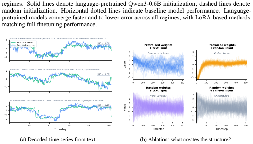
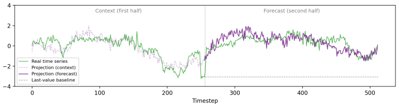
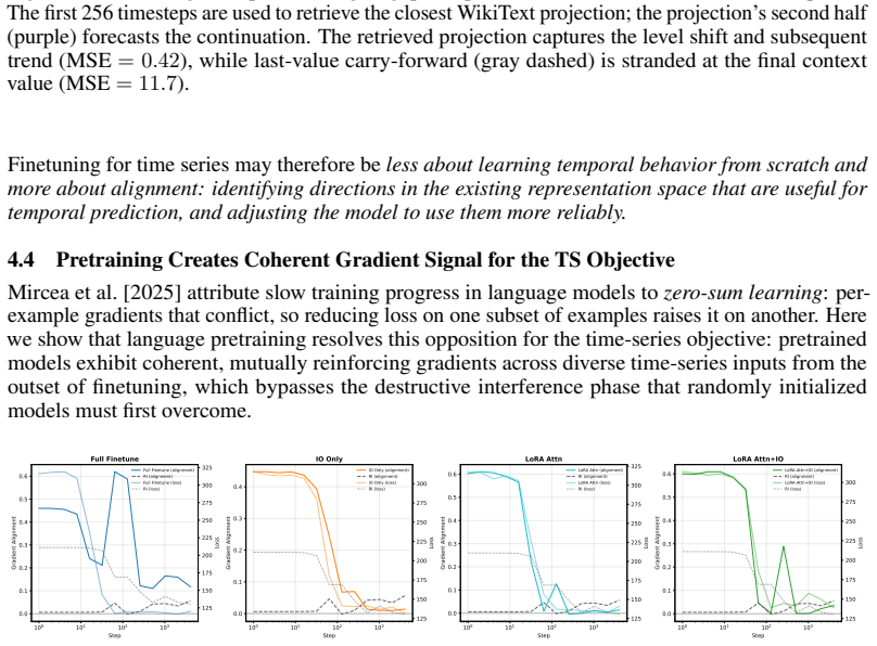
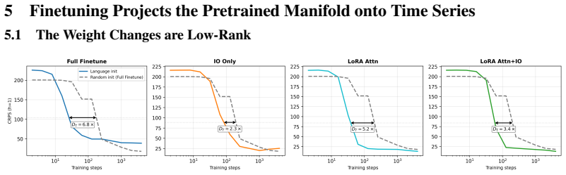
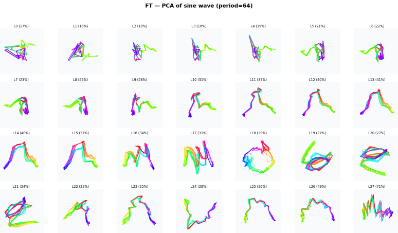
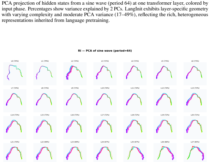
Cross-modal transfer arises because language pretraining preconditions time series training with a reusable manifold. A linear probe on frozen LLM states decodes realistic time-series trajectories without paired supervision, and retrieval in this projected space yields competitive forecasts, showing that structure and dynamics exist before finetuning. Pretrained initialization also improves optimization, producing coherent gradients and a highly anisotropic loss landscape unlike random initialization. Finetuning then acts as low-dimensional alignment, reusing existing directions rather than learning temporal primitives from scratch, as evidenced by low-rank updates, subspace alignment, and共享
What carries the argument
The reusable manifold induced by language pretraining in the LLM's hidden states, which supports linear decoding of time series trajectories and low-rank alignment during finetuning.
Load-bearing premise
The observed structure in frozen LLM states and the low-rank nature of finetuning updates are caused by language pretraining creating a generalizable manifold, rather than by model architecture, optimizer choices, or properties of the time-series datasets themselves.
What would settle it
If a transformer trained from random initialization on the same time series tasks shows comparable linear probe performance for decoding realistic trajectories and similar low-rank finetuning updates, the claim that language pretraining specifically shapes the manifold would be falsified.
Figures


read the original abstract
Can language-pretrained transformers become effective time-series forecasters, and why? In this paper, we show that cross-modal transfer arises because language pretraining preconditions time series training with a reusable manifold. A linear probe on frozen LLM states decodes realistic time-series trajectories without paired supervision, and retrieval in this projected space yields competitive forecasts, showing that structure and dynamics exist before finetuning. Pretrained initialization also improves optimization, producing coherent gradients and a highly anisotropic loss landscape unlike random initialization. Finetuning then acts as low-dimensional alignment, reusing existing directions rather than learning temporal primitives from scratch, as evidenced by low-rank updates, subspace alignment, and shared features for periodicity, trend, and repetition. Together, these results support a geometric account of LLM-to-time-series transfer: language pretraining builds the manifold, and finetuning projects numerical dynamics onto task-relevant directions.
Editorial analysis
A structured set of objections, weighed in public.
Referee Report
Summary. The manuscript claims that language pretraining of transformers preconditions time-series training by building a reusable manifold. Evidence includes linear probes on frozen LLM states decoding realistic trajectories without paired supervision, retrieval in the projected space producing competitive forecasts, pretrained initialization yielding coherent gradients and anisotropic loss landscapes unlike random starts, and finetuning consisting of low-rank updates that align to existing directions for periodicity, trend, and repetition rather than learning primitives from scratch.
Significance. If the results hold, the work supplies a geometric account of cross-modal transfer with concrete empirical support from linear probing, retrieval forecasts, and low-rank update analysis. These elements constitute reproducible strengths that could inform initialization strategies and adaptation methods for sequential tasks.
major comments (2)
- [Abstract and experiments on frozen states / low-rank updates] Abstract and experiments contrasting pretrained vs. random initialization: the claim that language pretraining specifically builds the reusable manifold requires isolating the pretraining corpus from architecture and optimizer effects. The current design does not hold the transformer architecture fixed while ablating the pretraining data (language corpus vs. synthetic sequences vs. none), leaving open that low-dimensional directions for periodicity/trend and coherent gradients could arise from any transformer on sequential data under standard optimizers.
- [Finetuning analysis] § on finetuning updates and subspace alignment: the interpretation that finetuning reuses existing directions rather than learning temporal primitives rests on low-rank updates and shared features, but without controls that vary only the pretraining objective while matching architecture and data statistics, the geometric account remains compatible with architecture-driven priors.
minor comments (2)
- [Abstract] The abstract packs multiple distinct experiments into a single paragraph; separating the linear-probe, retrieval, and optimization results into distinct sentences would improve readability.
- Notation for the projected space and manifold dimensions is introduced without an explicit definition or reference to a methods subsection; adding a short notation table or equation would clarify reuse across sections.
Simulated Author's Rebuttal
We thank the referee for the constructive feedback and positive evaluation of the work's significance. We address each major comment below with clarifications on the experimental design and scope of our claims, while indicating targeted revisions to strengthen the manuscript.
read point-by-point responses
-
Referee: [Abstract and experiments on frozen states / low-rank updates] Abstract and experiments contrasting pretrained vs. random initialization: the claim that language pretraining specifically builds the reusable manifold requires isolating the pretraining corpus from architecture and optimizer effects. The current design does not hold the transformer architecture fixed while ablating the pretraining data (language corpus vs. synthetic sequences vs. none), leaving open that low-dimensional directions for periodicity/trend and coherent gradients could arise from any transformer on sequential data under standard optimizers.
Authors: We agree that fully isolating the language corpus would require additional controls such as pretraining the same transformer architecture on synthetic sequences. Our current experiments hold architecture and optimizer fixed while contrasting language-pretrained initialization against random initialization, which isolates the contribution of language pretraining to the observed manifold properties (linear probe decoding, retrieval forecasts, gradient coherence, and anisotropic landscapes). We will revise the abstract and introduction to clarify that our claims concern the sufficiency of language pretraining for building a reusable manifold rather than exclusivity over all possible pretraining regimes, and we will add a limitations paragraph discussing synthetic pretraining ablations as valuable future work. revision: partial
-
Referee: [Finetuning analysis] § on finetuning updates and subspace alignment: the interpretation that finetuning reuses existing directions rather than learning temporal primitives rests on low-rank updates and shared features, but without controls that vary only the pretraining objective while matching architecture and data statistics, the geometric account remains compatible with architecture-driven priors.
Authors: We acknowledge that architecture-induced priors could influence low-rank updates and subspace alignments in isolation. However, by comparing pretrained versus randomly initialized models under identical architectures, data statistics during finetuning, and optimizers, our results show differential behavior: pretrained models exhibit more coherent gradients, anisotropic loss landscapes, and low-rank updates aligned to periodicity/trend directions, while random starts do not. This differential evidence supports that language pretraining shapes the manifold. We will expand the finetuning analysis section to explicitly discuss architecture priors as a potential contributing factor and how the pretrained-versus-random contrast addresses the geometric account within the scope of our controls. revision: partial
Circularity Check
No circularity: claims rest on empirical contrasts between pretrained and random initializations
full rationale
The paper's derivation consists of experimental observations: linear probes on frozen LLM states decode trajectories, retrieval in the projected space produces forecasts, pretrained initialization yields coherent gradients and anisotropic landscapes unlike random starts, and finetuning produces low-rank updates with subspace alignment. These findings are obtained by direct measurement and comparison on the same models and datasets; they do not reduce to fitted parameters renamed as predictions, self-definitional loops, or load-bearing self-citations. No equations or uniqueness theorems are invoked that presuppose the target manifold structure, and the geometric interpretation is presented as a post-experimental account rather than a premise that forces the results. The account is therefore self-contained against the reported benchmarks.
Axiom & Free-Parameter Ledger
axioms (1)
- domain assumption The internal representations of a frozen LLM contain decodable temporal structure independent of any time-series supervision.
invented entities (1)
-
reusable manifold
no independent evidence
Reference graph
Works this paper leans on
-
[1]
(act=14.1)“. . . becoming later in the year by about two days every 243-year cycle. Transits usually occur in pairs, on nearly the same date eight years apart.”
-
[2]
(act=13.8)“In practice, forward premiums and discounts are quoted as annualized percentage deviations from the spot exchange rate. . . ”
-
[3]
The working age population of the town in 2011
(act=13.7)“Wages are reflective of the type of jobs available locally, including higher than average employ- ment in manufacturing and the public sector. The working age population of the town in 2011. . . ”
work page 2011
-
[4]
(act=13.7)“So for americium-241, the resistivity at 4.2 K increases with time from about 2 µOhm ·cm to 10 µOhm·cm after 40 hours, and saturates at about 16 µOhm·cm. . . ”
-
[5]
(act=13.7)“Falcon’s Fury can theoretically accommodate 800 riders per hour. Carbon-fiber wings buttress each end of a group of seats. . . ” The shared representation encodesquantitative magnitude and transition: literal level shifts in time series, and passages dense with measurements, unit conversions, and numerical comparisons in text. Feature 2469 (Lay...
-
[6]
(act=8.7)“. . . the mean locus of formation shifts westward to the Caribbean and Gulf of Mexico, reversing the eastward progression of June through August. Wind shear from westerlies increases substantially through November. . . ”
-
[7]
due to a combination of very high wind shear and dry air
(act=8.3)“. . . due to a combination of very high wind shear and dry air. By October 17, most of the deep convection associated with the system dissipated; however, a brief decrease in wind shear allowed Omar to re-strengthen. . . ”
-
[8]
The convective system organized into Tropical Depression Twenty-E on September 28
(act=8.1)“The wave continued westward and related thunderstorm activity increased during the following week. The convective system organized into Tropical Depression Twenty-E on September 28. . . ”
-
[9]
It strengthened at a moderate pace and reached hurricane intensity on October 18.”
(act=8.1)“A tropical wave moved across the northeast Pacific Ocean and formed a tropical depression south of Mexico on October 16. It strengthened at a moderate pace and reached hurricane intensity on October 18.”
-
[10]
(act=7.9)“. . . formation of Typhoon Chanchu in the western Pacific enhanced convective activity over the Bay of Bengal. By April 22, a trough developed along an axis from the southern Bay of Bengal eastward to the Andaman Sea.” The time-series patterns—volatile signals with sudden regime changes—mirror the physical phenomena de- scribed in the text: trop...
-
[11]
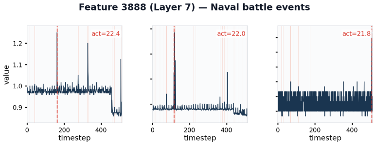
Admiral Tovey signalled his battlegroup
(act=10.1)“King George V had only 32 percent of her fuel left while Rodney had only enough fuel to continue the chase at high speed until 8:00 the following day. Admiral Tovey signalled his battlegroup. . . ”
-
[12]
(act=9.3)“At 7:20 on 19 July, the destroyer force spotted and was spotted by a pair of Italian light cruisers; Giovanni dalle Bande Nere and Bartolomeo Colleoni, which opened fire seven minutes later.”
-
[13]
The opposing ships began an artillery
(act=9.2)“Shortly before 16:00 the battlecruisers of I Scouting Group encountered the British 1st Bat- tlecruiser Squadron under the command of Vice Admiral David Beatty. The opposing ships began an artillery. . . ”
-
[14]
(act=9.2)“The eastern wind was not communicated to the aircraft, but was 270°, varying from 20 to 40 knots (37 to 74 km/h). The take-off started at 14:42:43. . . ”
-
[15]
(act=9.1)“. . . torpedo boat attacks and at 07:30, Burrough sent Eskimo and Somali back to help Manchester but they arrived too late, took on survivors. . . ” Both modalities encodesudden, precisely-located events: an anomalous spike at a single timestep in time series, and a precisely-timestamped combat event in text. Feature 2567 (Layer 8) — Missing / n...
-
[16]
(act=19.8)“. . . at the Royal Navy School of Flight Deck Operations at RNAS Culdrose. The following is an incomplete list of some of the surviving aircraft.”
-
[17]
(act=18.5)“ <unk>, <unk>, <unk>, <unk>, <unk>, Ulaid. Slightly later major groups included the Con- nachta,<unk>,<unk>. Smaller groups included the<unk>. . . ”
-
[18]
(act=18.0)“. . . he encountered bad weather, forcing him to return to Japan with heavy damage. Without waiting for Vizcaino, another ship—built in Izu by the Tokugawa shogunate. . . ” 4.(act=17.8)“Luke 9:<unk>-<unk>—κα`ι<unk>,<unk> <unk> <unk>πνε´υµατ oς<unk> <unk>. . . ”
-
[19]
(act=17.7)“. . . whom he married in the late 250s when she was 17 or 18 years old. The number of children Odaenathus had with his first wife is unknown and only one is attested.” The model representsabsent informationidentically across modalities: NaN values in time series and <unk> tokens in text both occupy the same region of representation space. E Cau...
work page 2024
discussion (0)
Sign in with ORCID, Apple, or X to comment. Anyone can read and Pith papers without signing in.