REVIEW 4 major objections 6 minor 44 references
Precise charge state distribution of projectile ions through solid targets
T0 review · 4 major / 6 minor · reviewed 2026-08-08 · deepseek-v4-flash
Pith's one-line read This paper claims that using four separate logistic curves for mean charge, one per projectile atomic-number group, yields charge-state distributions close to measured values for all solid targets in the 1-4 MeV/u range.
desk verdict A useful four-group logistic interpolation of published mean charge states, but the paper overclaims predictive precision because all parameters are fit and validated on the same Shima et al. data. read the letter →
The pith
A machine-rendered reading of the paper's core claim, the machinery that carries it, and where it could break.
The reading
What carries the argument
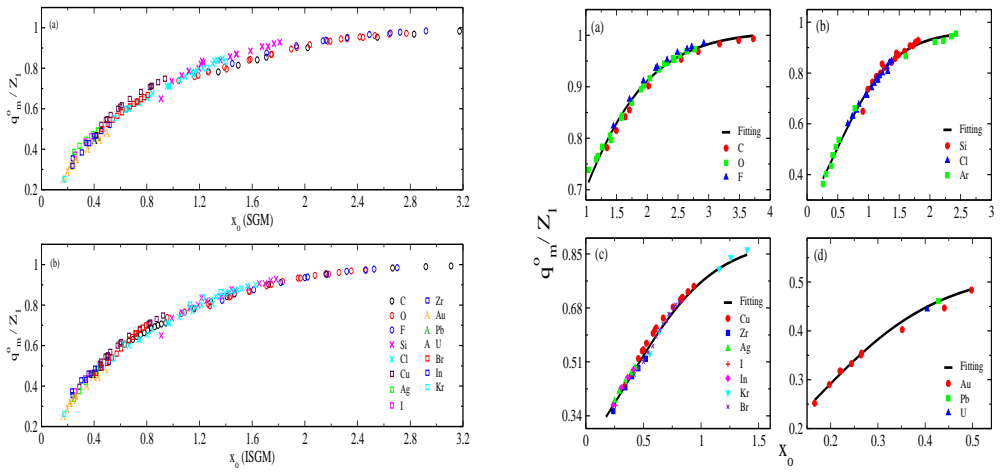
The engine of the model is a four-branch logistic description of the mean charge state. Using the Schiwietz-Grande reduced parameter $x_o$, a scaled projectile velocity that absorbs $Z_1$ and $Z_2$ dependence, the paper fits $q_o^m/Z_1$ to the logistic form $L/(1+\exp(-K(x_o-x')))$ separately for $Z_1 \le 10$, $10 < Z_1 \le 18$, $18 < Z_1 \le 54$, and $54 < Z_1 \le 92$. A table of 22 piecewise corrections in $Z_1$, $Z_2$, and energy adjusts these predictions for non-carbon targets. The resulting $q_o^m$ centers a Gaussian charge-state distribution whose width is set by the Novikov-Teplova formula $\Gamma(x_1)$ with $x_1 = q_o^m/Z_1$. This combination is what carries the argument: it converts a mean-charge estimate into a complete $F(q)$ without any experimental charge fractions.
What would settle it
A concrete check: refit Equations 16-19 and Table I on half of the data in Shima et al. and Ball et al., then compare predictions on the other half; if the held-out mean charges and widths scatter by more than the deviations shown in Fig. 9, the claimed precision is a fitting artifact.
Extended reading notes
Core claim
The central claim is that a single universal mean-charge formula is the wrong level of description for the intermediate-energy solid-target regime: the reduced parameter $x_o$ from Schiwietz and Grande organizes the data into four distinct bands, and each band needs its own logistic fit. The paper asserts that the four fitted curves (Eqs. 16-19) give mean charges $q_o^m$ in agreement with experiment on carbon targets, and that the addition of 22 piecewise target corrections (Table I) extends the agreement to heavy targets. With $q_o^m$ from this construction and the distribution width of Novikov and Teplova, a Gaussian ansatz for $F(q)$ yields charge-state distributions the authors find very close to the measured ones across the whole projectile range. The paper claims this supplies complete CSDs for $Z_1$ up to 92 in the 1-4 MeV/u energy range without using experimental charge fractions as input.
Load-bearing premise
The model assumes that four logistic curves plus 22 target corrections, all fitted to the Shima et al. carbon-target data, transfer to every solid target and every energy in the 1-4 MeV/u range without being tested on data that were not used in fitting.
Editorial extensions
If this is right
- Accelerator users could read off the full charge-state spectrum after a stripper foil for ions from carbon to uranium in the intermediate-energy range, not just the mean charge.
- Beams of non-dominant charge states, often needed for specific experiments, could be estimated without repeated calibration runs.
- The model offers an empirical benchmark against which fully theoretical CSD codes can be tested in the regime where heavier-than-Ni-like ions are hard to treat.
- Because the recipe is algebraic, it is suitable for online beam-dynamics and code-based accelerator planning.
Reading between the lines
- Not reported in the paper: the four logistic curves and the 22 target corrections are fitted to the same experimental set used for validation, so a leave-one-out or holdout test on unseen projectile-target-energy combinations would decide whether the model predicts or interpolates.
- A natural extension, not pursued here, is to test the same four-group logistic structure just outside the stated 1-4 MeV/u window; the piecewise target corrections would reveal whether the energy bands are physical or just fitting artifacts.
- The same Gaussian-plus-width construction could be applied to gaseous targets or to thinner foils before charge equilibrium is reached, domains where the structure of the corrections may need to change.
Editorial analysis
A structured set of objections, weighed in public.
Referee Report
Summary. The paper proposes an empirical model to compute mean charge states and charge-state distributions (CSDs) of projectile ions passing through solid targets in the 1-4 MeV/u energy range. The model divides projectiles into four atomic-number groups, fits a logistic function of the Schiwietz-Grande reduced parameter x0 to data from Shima et al. (Refs. [9,21]), adds 22 piecewise correction terms for heavy targets (Z2 >= 12) in Table I, and combines the resulting mean charge with the Novikov-Teplova width in a Gaussian to obtain F(q). The authors compare the resulting mean charges, widths, and CSDs with experimental values from the same Shima et al. data and report excellent agreement.
Significance. If the model could be validated out-of-sample, it would be practically useful: it offers an explicit procedure for estimating full CSDs without running a charge-exchange code, covers heavy ions up to uranium, and makes a concrete falsifiable claim that a single Gaussian with the Novikov-Teplova width reproduces F(q) for the full Z1 range. The paper also clearly identifies the limitation of the previous single-formula models for Z1 > 16. However, the current evidence is fit-quality evidence, not prediction evidence: no independent data set, holdout split, or cross-validation is used, and the four-group structure plus the many correction terms are chosen ad hoc from the same data. No uncertainty analysis is provided, so the claimed precision over the entire Z1-Z2-energy range is not established.
major comments (4)
- [Section IV and Section V] The validation is circular. The logistic parameters in Eqs. (16)-(19) and the 22 correction entries in Table I were chosen by fitting to the same Shima et al. experimental data (Refs. [9,21]) that are later compared in Figs. 7, 9, and 11-16. The reported agreement is therefore an in-sample residual metric, not a test of predictive accuracy. The authors should either compare with independent experimental data not used in the fitting or perform a holdout/cross-validation study (e.g., train on a subset of projectile-target-energy combinations and test on the remaining ones) before claiming precise prediction over the full range.
- [Section IV, Eq. (19)] The paper acknowledges that the group IV fit (54 < Z1 <= 92) is based on very few points: only Au at several energies and a few points for Pb and U. A three-parameter logistic fitted to such a sparse set cannot support the claim of precise prediction for all Z1 up to 92. Please provide parameter uncertainties, indicate the actual number of data points used, and either add more data or restrict the claimed validity range for group IV.
- [Section V, Eq. (10)] The RSM values (e.g., 0.0017 for C/Si) are computed on the same data used for fitting, so they quantify training residuals rather than prediction error. Moreover, no error bars are shown for the experimental data in Figs. 1, 7, and 9-16, and there is no propagation of uncertainties from the fitted parameters to the final F(q) values. Without such information, the stated precision cannot be evaluated.
- [Section II, Eq. (7)] The Novikov-Teplova width formula introduces extra empirical parameters (alpha = 0.23, beta = 0.32, and C as a function of Z1 and Z2) that themselves are fitted to experimental data. The paper does not state the fitting database for this formula or test whether it remains accurate for heavy targets and the heaviest projectile groups. This is load-bearing because the final CSD claim depends on both the new mean-charge model and this width formula.
minor comments (6)
- [Title page] There are spacing typos in the title and affiliations: 'throu gh' and 'In dia' should be corrected.
- [Section II, Eq. (9)] Equation (9) has an unbalanced parenthesis: the expression contains an extra closing bracket after (Z1^{−0.45} v1/v')^{-1/0.6}. Please check and correct the formula.
- [Section II, Eq. (14)] The exponent of Z2 in Eq. (14) is ambiguous ('Z_2^{-0.019Z - 0.52 v1/v0} / 1.68'); please clarify the intended power-law form and define all symbols in the equation.
- [Section IV, Eq. (15)] In Eq. (15), x' is called the midpoint, but the fitted constants in Eqs. (16)-(19) are not identified as x' values; please state explicitly which fitted parameter corresponds to x'.
- [Section V, Figs. 3-4 and 11-16] Many panels are very small and the projectile/target/energy labels are difficult to read, especially in Figs. 11-16. Please enlarge fonts and ensure each panel's labels are legible.
- [Abstract and Section IV] The abstract states the range as 1 MeV/u < E < 4 MeV/u, but several validation data points lie below 1 MeV/u (e.g., Cl on C at 0.688 MeV/u in Fig. 3 and Cu on C at 0.558 MeV/u in Fig. 4). Please reconcile the claimed energy range with the data used.
Circularity Check
The model's four-group logistic q_m curves and Table I corrections are fitted to the same Shima et al. data later used as the experimental benchmark, making the claimed CSD 'agreement' in-sample rather than predictive.
-
fitted input called prediction
[Section IV (Eq. 15) / Section V (Eqs. 16–19), Figs. 6, 7, 11–16]
"we first consider only the experimental data on the light (carbon) targets, which can be classified into four groups of projectile ions as follows: (a) Z1 ≤ 10, (b) 10 < Z1 ≤ 18, (c) 18 < Z1 ≤ 54, and (d) 54 < Z1 ≤ 92. The qm/Z1 are plotted as a function of the same reduced parameter xo as given in Eqn. (14) and all the four curves have been fitted with the standard logistic function as follows."
The parameters of Eqs. (16)–(19) are determined by fitting the Shima et al. experimental mean charge states [9,21] on carbon targets. Later, the same references [9,21] are used as the 'experiment' in Fig. 7 for q_m and in Figs. 11–16 for F(q). Consequently, the reported agreement is an in-sample property of the fitted logistic curves, not an independent prediction. The RSM values quoted (e.g., 0.0017 for C/Si) are fit residuals, not out-of-sample accuracy estimates.
-
fitted input called prediction
[Section IV, Table I; Section V, Fig. 8]
"However, the scenario with other than carbon targets as shown in Fig. 8 with solid line is not that good. To make it better, we have modified the equations 16 to 19 by adding certain correction terms as given in Table I. The comparison of the experimental data with such modified equations is shown with the dotted lines. A good agreement is observed between the experimental data and present estimates for all the groups."
The 22 piecewise correction entries in Table I are introduced after the solid-line model visibly deviates from the same Shima et al. data plotted in Fig. 8. Their coefficients and Z2/E thresholds are chosen to reduce the residual on those very data points, so the subsequent dotted-line 'good agreement' with the same points is a restatement of the fit. No held-out projectile-target-energy combination is used, so the transferability claim to Z2 ≤ 92 over the whole 1–4 MeV/u range is not tested by these comparisons.
full rationale
The paper's central new ingredient is the replacement of the single ISGM mean-charge formula by four logistic formulas, Eqs. (16)–(19), plus 22 ad hoc target corrections in Table I. The manuscript states explicitly that these formulas and corrections were obtained by fitting the experimental data of Shima et al. [9,21], and then the same data are used as the experimental benchmark in nearly every validation figure (Figs. 7, 8, 11–16). For carbon targets this is a direct instance of fitted input being called prediction: the logistic curves are least-squares fits to the q_m values that are later compared, so the agreement is by construction. For non-carbon targets, the Table I corrections were introduced only after Fig. 8 exposed systematic deviations from the same database, so the 'good agreement' after correction is likewise an in-sample residual rather than independent validation. The Gaussian distribution (Eq. 12) and the Novikov–Teplova width (Eq. 7) are external ingredients and are not themselves fitted in this paper; the width comparisons in Fig. 10 provide some independent support for that part of the model. However, the mean charge state is the central determinant of the CSD peak and the paper itself identifies q_m as 'our challenge.' Since that q_m is fitted to exactly the data used for validation, the headline claim of precise CSDs over the full Z1, Z2, and energy range is not independently established. This is a partial but substantial circularity, not a full identity of model and data because of the externally supplied Gaussian/NAT components and the genuine four-band classification attempt; nevertheless, the quantitative 'precision' claim reduces largely to a fit report.
Assumptions & free parameters
free parameters (6)
- Group 1 logistic parameters (L, K, x') =
L=1.007704, K=1.419686, x'=0.416069
- Group 2 logistic parameters (L, K, x') =
L=0.966005, K=2.117365, x'=0.454663
- Group 3 logistic parameters (L, K, x') =
L=0.901506, K=2.674817, x'=0.368080
- Group 4 logistic parameters (L, K, x') =
L=0.525255, K=7.609263, x'=0.170544
- Table I target corrections =
22 piecewise coefficients (0.8, 1.5, 0.2, 0.7, -1.4, 0.05, 0.2, 1.2, -0.1, -0.05, -0.2, 1.2, -1.2, -0.3, -1, -2, -0.1…
- Z1 group boundaries =
10, 18, 54
assumptions (5)
- domain assumption The reduced parameter xo of SGM (Eq. 14) is a sufficient scaling variable for all solid targets and ion species.
- domain assumption The charge state distribution is Gaussian with width given by Novikov and Teplova (Eq. 7).
- domain assumption The exit beam energies are correctly computed with the SRIM code.
- ad hoc to paper The four-group split and the piecewise correction terms are appropriate.
- domain assumption The experimental data sets from Refs [9,21] are accurate and internally consistent.
Cite this review
Pith. "Pith review of Precise charge state distribution of projectile ions through solid targets." pith.science (2026). https://pith.science/paper/CGG46XPH
@misc{pith2026250204831,
  author       = {Pith},
  title        = {Pith review of: Precise charge state distribution of projectile ions through solid targets},
  year         = {2026},
  howpublished = {\url{https://pith.science/paper/CGG46XPH}},
  note         = {Machine review of arXiv:2502.04831}
}
abstract
The charge state distribution (CSD) of the projectile ions through solid targets in the intermediate energy range (1 MeV/u $<$ E $<$ 4 MeV/u) has a major impact on the collision of the ion atom and accelerator physics. We explore the mean charge states taken from the empirical formula [Schiwietz $et~al.$, Nucl. Inst. Meths. {\bf 225}, 4(2004)] are only good for projectile ions with $Z_1 \le 16$. To solve this issue, we develop a model in which instead of a single formula, if we employ four formulae, the comparative picture between experimental and empirical data becomes impressive. Furthermore, the CSDs with the mean charge state so obtained and the Gaussian distribution function having distribution width given by [Novikov and Teplove, Phys. Lett. {\bf378}, 1286(2014)] compare well with the experimentally measured CSDs for the entire range of projectile ions. We believe that precise CSDs will be highly useful in both ion-atom collision and accelerator physics.
Figures


Figures from the paper (7 more)


Reference graph
Works this paper leans on
-
[1]
The exit energy is estimated by deducting the ion energy loss in the foil calculated using the SRIM package [23] from the incident beam energy. Here, one can see that both these qo m and Γ agree well with the experimental data for the lighter heavy ions up to Z1 = 16. However, the picture is not the same for the heavy ions Z1 > 16. To check whether Nikola...
-
[2]
S. Chatterjee, P. Sharma, S. Singh, M. Oswal, S. Kumar, C. Montanari, D. Mitra, and T. Nandi, Physical Review A 104, 022810 (2021)
work page 2021
-
[3]
06 xo + 4 + 7. 4 xo + x4 o (2) Here the reduced parameter xo is written in terms of projectile velocity ( v1), projectile atomic number Z1, and target atomic number Z2 as follows xo = c1 ( ¯v c2 ·1. 54 ) ( 1+ 1.83 Z1 ) (3) ¯v = Z −0. 543 1 ( v1 vo ) (4) 3 3 4 5 6 0 0.2 0.4 0.6 ISGM Expt. Expt. Fit 2 4 6 8 0 0.2 0.4 0.6 4 5 6 7 8 0 0.2 0.4 0.6 5 6 7 8 9 0 ...
-
[4]
for different projectile ions ( Z1 ≤ 17) and various solid targets at diverse energies are compared with the corresponding experimental results. c1 = 1 − 0. 26 exp ( − Z2 11 ) exp ( − (Z2 − Z1)2 9 ) (5) c2 = 1 + 0 . 030 ¯v ln(Z2) (6) where vo is the Bohr velocity (2 . 19 × 106m/s ). Next, the distribution width Γ is taken from Novikov and Teplova [22] (NAT...
-
[5]
058.Z 1 + 0. 00048.Z 1.Z 2. Next, we have compared the mean charge state qo m as obtained from ISGM [12] and the width of the charge state distribution Γ from Novikov and Teplova [22] (NAT) with the corresponding experimental data [9, 21] as a function of the energy of emergence in Fig
-
[6]
This fitting gives us a clear pic- ture to obtain qo m well and yields the fitting equations 16 to 19 for any ion beams on the carbon target. A rep- resentative comparison of experimental qo m (red cross) 0 0.3 0.6 Present 0 0.3 0.6 0 0.3 0.6 0 0.3 0.6 00.20.40.6 0.8 Expt. 0 0.3 0.6 0 0.3 0.6 0 0.3 0.6 0 0.3 0.6F(q) 0 0.3 0.6 0 0.3 0.6 0 0.3 0.6 0 0.3 0.6 0...
-
[7]
Furthermore, we know that ISGM is good for light ion regime Z1 ≤ 16
It shows clearly that the present model best agrees with the experimental data. Furthermore, we know that ISGM is good for light ion regime Z1 ≤ 16. To check whether present model predictions for qo m in this region are even better than ei- ther SGM or ISGM, we have found out the RSM values of SGM, ISGM, and present model for two representa- tive cases (a...
-
[8]
We see that the empirical for- mula for F(q) fits well with the experimental data [9, 21] except for two cases (i) and (l). In both cases, Cl is the 1 1.5 2 2.5 3 3.5 4 0.7 0.8 0.9 1 Fitting C O F 0 0.5 1 1.5 2 2.5 3 0.4 0.6 0.8 1 Fitting Si Cl Ar 0 0.5 1 1.5 xo 0.34 0.51 0.68 0.85q o m/ Z1 Fitting Cu Zr Ag I In Kr Br 0.2 0.3 0.4 0.50.2 0.3 0.4 0.5 Fitting...
Show all 44 references
-
[9]
4 - (h), (i), (k), the other 17 data sets show a clear mismatch between the empirical and experimen- tal CSD
Except for a few cases in Fig. 4 - (h), (i), (k), the other 17 data sets show a clear mismatch between the empirical and experimen- tal CSD. To find the real cause of this disagreement, we employed the same method using Γ from Novikov and Teplova [22] and the Gaussian charge st...
-
[10]
52 1 Z −0
The parameter xo for SGM [11] is given as xo = (v1/v oZ −0. 52 1 Z −0. 019Z− 0.52 1 v1/v o 2 / 1. 68)1+1. 8/Z 1 (14) We revealed that Fig.5(a) exhibits a distinctive four-band pattern in the data, which is not observed in Fig. 5(b). Exactly, this was the objective of ISGM. How...
-
[11]
Specifically, the width parameter here makes it obvious that the model cannot predict F(q) independently
remains valid here too, but that formula contains the charge state fractions (F(q)) as follows Γ = [ ∑ q (q − qo m)2F (q)]1/ 2 (1) Hence, these formulae can only be used to calculate the CSD if F(q) is also known and it is possible from the ex- perimental data only. Specificall...
-
[12]
To examine which one of these agrees better in this comparison, we have tested the data by using a quantity called relative sum metrics (RSM)
and NAD (blue) [19] with the experimental mean charge state [9, 21] of projectile ions through solid tar- gets (red cross) seems to look quite similar. To examine which one of these agrees better in this comparison, we have tested the data by using a quantity called relative s...
-
[13]
The qo m for the projectile ions Z1 ≤ 10 (call it qo m1 ) can be obtained by using the em- pirical formula as follows qo m1 = Z1
and all the four curves have been fitted with the standard logistic function as follows qo m Z1 = L 1 + exp(− K(xo − x′)) (15) where x′ is the midpoint of the xo value, L is the supre- mum of the values of the function and K is the logistic growth rate of the curve. The qo m fo...
-
[14]
The reason for this consideration of the earlier xo pa- rameter is quite clear from Fig
from this instance. The reason for this consideration of the earlier xo pa- rameter is quite clear from Fig. 5(a); the data constitute a wide-spread band, and a single fitted line is too sim- ple to provide fairness to such data. Furthermore, we 7 0 1 2 3 4 5 6 7-4 -3 -2 -1 0 1...
-
[15]
419686(xo − 0
007704 1 + exp(− 1. 419686(xo − 0. 416069)) . (16) Similarly, the qo m for the projectile ions 10 < Z 1 ≤ 18 (call it qo m2 ), 18 < Z 1 ≤ 54 (call it qo m3) and 54 < Z 1 ≤ 92 10 20 30 40 50 600 0.4 0.8 1.2 Present Expt. 90 180 270 360 450 540 1 2 3 36 48 60 72 84 96 1080 0.5 1...
-
[16]
117365(xo − 0
966005 1 + exp(− 2. 117365(xo − 0. 454663)) , (17) qo m3 = Z1
-
[17]
674817(xo − 0
901506 1 + exp(− 2. 674817(xo − 0. 368080)) (18) and qo m4 = Z1
-
[18]
609263(xo − 0
525255 1 + exp(− 7. 609263(xo − 0. 170544)) . (19) There is quite a sufficient number of data for fitting the curve of Fig. 6(a)-(c), but the data available for fitting the curve of Fig. 6(d) are not many. Only data exist with Au at several energies and a few points for Pb and U p...
-
[19]
9 that the 9 0 0.2 0.4 Present 0 0.2 0.4 Expt
We can clearly see from Fig. 9 that the 9 0 0.2 0.4 Present 0 0.2 0.4 Expt. 0 0.2 0.4 0 0.2 0.4 0 0.2 0.4 0 0.2 0.4 0 0.2 0.4 0 0.2 0.4 0 0.2 0.4 0 0.2 0.4 0 0.2 0.4F(q) 0 0.2 0.4 0 0.2 0.4 0 0.2 0.4 0 0.2 0.4 0 0.2 0.4 0 0.2 0.4 0 0.2 0.4 8 10 12 14 q 0 0.2 0.4 8 10 12 14 0 0...
-
[20]
16-19 to obtain charge-state fraction values
and use qo m from Eqns. 16-19 to obtain charge-state fraction values. An excellent agreement between theoret- ical and experimental CSD can be seen in Fig. 11, which represents the graphs of F (q) versus q for the 12C and 0 0.2 0.4 Present 0 0.2 0.4 Expt. 0 0.2 0.4 0 0.2 0.4 0...
-
[21]
Here also, our predictions for CSD give very good agreement as shown for cases of 19F , 28Si, 10 0 0.2 Present 0 0.2 Expt. 0 0.2 0 0.2 0 0.2 0 0.2 0 0.2 0 0.2 0 0.2F(q) 0 0.2 0 0.2 0 0.2 0 0.2 0 0.2 0 0.2 0 0.2 8 12 16 20 24 q 0 0.2 12 16 20 24 28 32 0 0.2 Cu on C Cu on Al Cu ...
-
[22]
and NAD (blue plus) [19]. as heavy ions in the intermediate energy range are used to pass through the charge stripper to have higher charge states, so that higher energy will be obtained from the booster stage of the large accelerators. On this ground, empirical formulae may fi...
-
[23]
Sharma and T
P. Sharma and T. Nandi, Physical Review Accelerators and Beams 22, 034501 (2019)
2019
-
[24]
Chatterjee, S
S. Chatterjee, S. Kumar, S. Kumar, M. Oswal, B. Mo- hanty, D. Mehta, D. Mitra, A. Mendez, D. Mitnik, C. Montanari, et al. , Physica Scripta 97, 045405 (2022)
2022
-
[25]
M. Kaur, S. Kumar, and T. Nandi, Phys. Rev. A 108, 052817 (2023)
2023
-
[26]
Sharma and T
P. Sharma and T. Nandi, Physics of Plasmas 23, 083102 (2016)
2016
-
[27]
Maidikov, N
V. Maidikov, N. Surovitskaya, N. Skobelev, and W. Neubert, Nuclear Instruments and Methods in Physics Research 192, 295 (1982)
1982
-
[28]
BETZ, Rev
H.-D. BETZ, Rev. Mod. Phys. 44, 465 (1972)
1972
-
[29]
Shima, T
K. Shima, T. Ishihara, and T. Mikumo, Nuclear Instru- ments and Methods in Physics Research 200, 605 (1982)
1982
-
[30]
Shima, T
K. Shima, T. Mikumo, and H. Tawara, Atomic Data and Nuclear Data Tables 34, 357 (1986)
1986
-
[31]
Shima, N
K. Shima, N. Kuno, M. Yamanouchi, and H. Tawara, Atomic Data and Nuclear Data Tables 51, 173 (1992)
1992
-
[32]
Schiwietz and P
G. Schiwietz and P. Grande, Nuclear Instruments and Methods in Physics Research Section B: Beam Interac- tions with Materials and Atoms 175, 125 (2001)
2001
-
[33]
Schiwietz, K
G. Schiwietz, K. Czerski, M. Roth, F. Staufenbiel, and P. Grande, Nuclear Instruments and Methods in Physics Research Section B: Beam Interactions with Materials and Atoms 225, 4 (2004)
2004
-
[34]
Chatterjee, P
S. Chatterjee, P. Sharma, D. Mitra, and T. Nandi, arXiv preprint arXiv:2103.08299v4 (2021)
2021 arXiv
-
[35]
J. P. Rozet, A. Chetioui, P. Piquemal, D. Vern- het, K. Wohrer, C. Stephan, and L. Tassan-Got, Journal of Physics B: Atomic, Molecular and Optical Physics 22, 33
-
[36]
Rozet, C
J. Rozet, C. St´ ephan, and D. Vernhet, Nuclear Instruments and Methods in Physics Research Sectio n B: Beam
-
[37]
Lamour, P
E. Lamour, P. D. Fainstein, M. Galassi, C. Prigent, C. A. Ramirez, R. D. Rivarola, J.-P. Rozet, M. Trassinelli, and D. Vernhet, Phys. Rev. A 92, 042703 (2015)
2015
-
[38]
Swami and T
D. Swami and T. Nandi, Radiation Physics and Chemistry 153, 120 (2018)
2018
-
[39]
Scheidenberger, T
C. Scheidenberger, T. St¨ ohlker, W. Meyerhof, H. Geis- sel, P. Mokler, and B. Blank, Nuclear Instruments and Methods in Physics Research Section B: Beam Interac- tions with Materials and Atoms 142, 441 (1998)
1998
-
[40]
Nikolaev and I
V. Nikolaev and I. Dmitriev, Physics Letters A 28, 277 (1968)
1968
-
[41]
H. D. Betz and L. Grodzins, Physical Review Letters 25, 211 (1970)
1970
-
[42]
G. Ball, T. Alexander, H. An- drews, W. Davies, and J. Forster, Nuclear Instruments and Methods in Physics Research Sectio n B: Beam
-
[43]
Novikov and Y
N. Novikov and Y. A. Teplova, Physics Letters A 378, 1286 (2014)
2014
-
[44]
J. F. Ziegler, M. D. Ziegler, and J. P. Biersack, Nuclear Instruments and Methods in Physics Research Section B: Beam Interactions with Materials and Atoms 268, 1818 (2010)
2010
Reviewed August 8, 2026 · model on record in the stance chip above.
Discussion (0). Continue with ORCID to comment.