REVIEW 3 major objections 6 minor 45 references
End of the constant-roll inflation, and the reheating temperature
T0 review · 3 major / 6 minor · reviewed 2026-08-14 · deepseek-v4-flash
Pith's one-line read The paper shows that multiplying the constant-roll potential by a function that switches on near a minimum lets constant-roll inflation end and reheat the Universe, and it derives the reheating temperature from the observed perturbation…
desk verdict The exit mechanism works, but the reheating-temperature formula has a load-bearing exponent error; don't trust the numbers, do trust the qualitative mechanism. read the letter →
The pith
A machine-rendered reading of the paper's core claim, the machinery that carries it, and where it could break.
The reading
What carries the argument
The load-bearing object is the modified potential of eq. (32), $V_{\rm new}(\phi)=f(\phi)V_{\rm old}(\phi)$, with $f\simeq1$ in the inflationary epoch and $V_{\rm new}\simeq \Lambda(\phi-\phi_{\rm min})^q$, $q$ even, near the minimum. It carries the argument because $f$ converts the unending constant-roll trajectory into an oscillatory phase: $\phi_{\rm end}$ is set by the condition $\lambda(\phi_{\rm end}-\phi_{\rm min})^q\simeq1$, and the oscillating field behaves like matter with equation-of-state parameter $w=(q-2)/(q+2)$. Equation (66) is the working identity: it collects the e-fold budget $N=\ln(H_*/k_0)$ from the four eras and inverts it for $T_{\rm reh}$, with $H_*$ fixed through the power-spectrum normalization (50). The correction factor $\xi=\frac12(f'/f)^2$ stays small in the example, so the constant-roll predictions for $n_s$ and $r$ are preserved.
What would settle it
One concrete test is to compute the effective equation of state during reheating from first principles for the paper's example potential, $V_{\rm new}(\phi)=f(\phi)V_{\rm old}(\phi)$ with $f=1-e^{-30(\phi-6)^2}$ and $\beta=0.015$ in Planck units, using a lattice preheating simulation; inserting the simulated $\bar w_{\rm eff}$ into eq. (66) gives a definite $T_{\rm reh}$, and if that value falls outside the few-times-$10^{15}$ GeV band shown in figs. 11–13, the model's reheating prediction is wrong. A measurement of the primordial gravitational-wave background from preheating, or a cosmological bound on the reheating temperature, would provide the same test without needing the microphysics.
Extended reading notes
Core claim
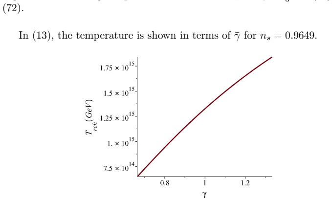
The paper's central claim is that the apparent dead end of constant-roll inflation—the roll never stops, so there is no natural reheating—can be removed by extending the potential to $V_{\rm new}(\phi)=f(\phi)V_{\rm old}(\phi)$ with $f\simeq 1$ during inflation and $f$ dropping to zero at $\phi_{\rm min}$. The field then leaves inflation at a computable $\phi_{\rm end}$ and oscillates around $\phi_{\rm min}$; near the minimum the potential behaves as $V_{\rm new}\simeq \Lambda(\phi-\phi_{\rm min})^q$ with even $q$, and the oscillation reheats the Universe. Equating the total e-fold number from horizon exit to today with the sum of the constant-roll, reheating, radiation, and recombination contributions gives the reheating temperature (66), with $H_*$ fixed by the curvature power spectrum. In the explicit example $f(\phi)=1-e^{-\lambda(\phi-\phi_{\rm min})^q}$ with $\lambda=30M_P^{-2}$, $\phi_{\rm min}=6M_P$, $q=2$, $\beta=0.015$, inflation ends after about 42 e-folds and the reheating temperature is within a few orders of magnitude of $10^{16}$ GeV, growing with $\bar\gamma=\bar w_{\rm eff}+1$ and changing by only about 0.1% across the observed range of $n_s$.
Load-bearing premise
The load-bearing premise is that the whole reheating era can be represented by a single effective equation-of-state parameter $\bar w_{\rm eff}$ (eqs. 55–56) that is never derived from the inflaton's interactions or fixed by data; every numerical reheating temperature scales with this input.
Editorial extensions
If this is right
- The constant-roll model that fits the observed perturbation spectra can be evolved all the way past inflation, so exit and reheating need not be imposed by hand.
- For the example parameters, $T_{\rm reh}$ changes by only about 0.1% as $n_s$ runs across its observed 1-$\sigma$ range, making the temperature a sharp prediction once the post-inflationary equation of state is fixed.
- The predicted reheating temperature sits a few orders of magnitude below the grand-unification scale, in line with the usual assumption that reheating happens before or at the scale of grand unification.
- The final state at $\phi_{\rm min}=6M_P$ is an attractor for all initial conditions with $0<\phi(0)\le6M_P$, so the reheating history is insensitive to the field's initial data.
- Because the corrections to $n_s$ and $r$ are controlled by the small quantity $\xi$, the observational success of the base constant-roll potential carries over to the extended model.
Reading between the lines
- If the inflaton's decay products and couplings were specified, a lattice or analytic preheating computation could replace the free parameter $\bar w_{\rm eff}$ with a number; the temperature formula (66) would then become a sharp prediction rather than a curve family.
- The same $f(\phi)$ construction is not tied to the particular potential (19): any never-ending constant-roll or non-attractor stage could be ended by inserting a factor that vanishes at a nearby minimum before $V_{\rm old}$ becomes negative.
- A future detection of a stochastic gravitational-wave background from preheating would probe the oscillatory stage directly and could select which value of $\bar\gamma$ actually operated, testing the model against its own temperature curves.
- The near-insensitivity of $T_{\rm reh}$ to $n_s$ is specific to this model; applying the same e-fold counting to slow-roll models amplifies small changes in $n_s$, so the comparison offers a way to distinguish the two frameworks observationally.
Editorial analysis
A structured set of objections, weighed in public.
Referee Report
Summary. This paper proposes a modification of the constant-roll inflaton potential, V_new(φ)=f(φ)V_old(φ) with f(φ)≈1 during inflation, so that constant-roll inflation ends and the inflaton oscillates around a minimum, reheating the Universe. The authors split the post-inflationary history into inflation, reheating, radiation, and recombination, and use the e-fold consistency condition N=ln(H_*/k_0) to solve for the reheating temperature in terms of Planck-normalized H_*, the constant-roll parameters β and M, the position φ_end, and an effective equation-of-state parameter w_eff. A numerical example with f(φ)=1−exp[−λ(φ−φ_min)^q] demonstrates exit and oscillation, and the paper plots T_reh versus γ and n_s.
Significance. If the quantitative derivation were correct, the paper would supply a useful complete inflation-reheating history for a constant-roll model and would show that T_reh is only weakly sensitive to n_s in this class of models. The mechanism for ending constant-roll inflation is coherent, the numerical example is explicit, and the calculation is not circular: H_* is fixed by the Planck-normalized spectrum and the constant-roll background comes from previous work. However, the central reheating-temperature formula contains an algebraic error that invalidates the reported numerical temperatures, and the result is also conditional on a free effective EoS parameter. With corrected algebra and a more transparent treatment of the EoS dependence, the paper could be publishable.
major comments (3)
- [Sec. 3.4, Eqs. (55), (59), (64), (66)] There is an inconsistency between the definition of the reheating e-fold number and the assembled formula. Eq. (55) defines N2 = −(1/(3γ)) ln(ρ_reh/ρ_end), and Eq. (59) is consistent with that, giving e^{N2} = (ρ_end/ρ_reh)^{1/(3γ)}. However, Eq. (64) contains the factor (3M_P^2 H^2(φ_end)/((g_reh/30)π^2 T_reh^4))^{3γ}, i.e. the density ratio raised to 3γ instead of 1/(3γ). Solving the correctly assembled equation for T_reh yields the exponent 3γ/(3γ−4), not 1/(12γ−1) as in Eq. (66); the sign of the correct exponent changes for γ<4/3. Since Figs. 11–13 and the conclusion that T_reh is a few orders of magnitude below the GUT scale are computed from Eq. (66), those quantitative results do not follow from the model as written.
- [Sec. 4, Eq. (69)] The position φ_end at which inflation ends is fixed by the order-of-magnitude criterion λ(φ_end−φ_min)^q ≈ 1 rather than by solving the background dynamics (2)–(4) with the modified potential (32) and (68). This matters because N1 in Eq. (37), H(φ_end) in Eq. (57), and therefore T_reh in Eq. (66) all depend on φ_end. The paper should either derive φ_end from the numerical solution or quantify how much T_reh changes under the uncertainty in this estimate.
- [Sec. 3.2, Eq. (56)] The effective EoS parameter w_eff (equivalently γ = w_eff + 1) is introduced as an average over the reheating era but is never determined from the inflaton's couplings or from an explicit preheating calculation. Because Eq. (66) depends on γ through a power law, all numerical temperatures reported in Figs. 11–13 are conditional on this free input. The paper acknowledges that a precise determination is not currently feasible, but the abstract and conclusion should not present T_reh as a model-independent estimate based on astrophysical data.
minor comments (6)
- [Sec. 2, after Eq. (28)] The sentence 'For β < 0, and for the potential (19)' appears to be a typo: Eq. (28) uses H = M coth(−βM t), which is the β<0 solution corresponding to potential (14), not potential (19).
- [Fig. 2 caption] The caption says 'The plot of (14) for β=0.015', but Eq. (14) is the β<0 potential; the plotted potential for β>0 is Eq. (19).
- [Sec. 3.1, after Eq. (37)] The text reads 'So NI depends on φ∗, φend, and β'; the subscript should be N1 for consistency with Eq. (34).
- [Sec. 4, final paragraph] The statement 'we numerically solved (2) and (44)' likely refers to the Friedmann and Klein-Gordon equations (2) and (4), not Eq. (44), which is the power-spectrum amplitude.
- [Eq. (66) and surrounding text] The quantities ilde T_reh, ilde T_CMB, and ilde k_0 are dimensionless (in units of M_P), but this is never stated explicitly; the authors should define these reduced variables before Eq. (66).
- [References] Reference [35] contains a typo in the journal citation: 'JCAP 11 02, 021' should be 'JCAP 1102, 021'.
Circularity Check
No significant circularity: T_reh is solved from an e-fold consistency condition, the inflationary background comes from external constant-roll literature, and the self-citations are not load-bearing.
full rationale
The paper's central quantitative prediction, the reheating temperature, is not equivalent to an input by construction. The inflationary background and its perturbation normalization are taken from the external constant-roll works [19,20] and from Planck data (51); the modified potential V_new=f(phi)V_old is a model-building ansatz, and phi_end is estimated via the order-one criterion (69), not fitted to the reheating temperature later obtained. The reheating temperature appears as the unknown in the e-fold consistency equation obtained by equating (64) and (65), so it is a derived quantity rather than an inserted datum. The acknowledged limitation that w_eff cannot be precisely computed until inflaton interactions are identified (Sec. 3.2) is an underdetermination of an input parameter, not a circular step. The self-citations [37,38,43] are used only as references for the standard reheating-e-fold method, which is also attributed to [33,42]; the argument does not reduce to a self-citation chain. The algebraic exponent mismatch between Eq. (55) and Eq. (64) identified in the review context is a correctness or consistency concern, not a circularity: correcting the algebra would still leave T_reh as the output of the consistency equation. Overall, the derivation chain is self-contained in the sense required by the circularity rubric, though the numerical reheating-temperature claim carries separate model-dependence and potential algebraic risks.
Assumptions & free parameters
free parameters (7)
- beta (constant-roll parameter) =
0.015 in the numerical example
- M (constant-roll mass scale) =
about 10^-5 M_P in the example
- phi_min (minimum of modified potential) =
6 M_P
- lambda (f(phi) steepness) =
30 M_P^-2
- q (order of potential minimum) =
2
- phi_star (initial field value) =
3 M_P
- bar_gamma (effective EoS parameter during reheating) =
scanned, not fixed
assumptions (6)
- domain assumption FLRW metric and canonical scalar field action (1) describe inflation and reheating.
- domain assumption The constant-roll condition ddot_phi = beta H dot_phi holds during inflation.
- domain assumption The curvature perturbation power spectrum from Motohashi, Starobinsky and Yokoyama [19] applies to the constant-roll phase.
- domain assumption f(phi) is negligible at CMB horizon exit, so ns and r from the unmodified constant-roll potential remain valid.
- domain assumption The reheating era is characterized by a single constant average EoS parameter w_eff.
- domain assumption Instantaneous transition to radiation domination at t_reh with entropy conservation afterwards.
Cite this review
Pith. "Pith review of End of the constant-roll inflation, and the reheating temperature." pith.science (2026). https://pith.science/paper/J45QOIDT
@misc{pith2026190804266,
  author       = {Pith},
  title        = {Pith review of: End of the constant-roll inflation, and the reheating temperature},
  year         = {2026},
  howpublished = {\url{https://pith.science/paper/J45QOIDT}},
  note         = {Machine review of arXiv:1908.04266}
}
read the original abstract
By extending the potential, we propose a mechanism for the end of the constant-roll inflation and the subsequent reheating phase in the FLRW space-time. Based on astrophysical data, we estimate the Universe reheating temperature.
Figures


Figures from the paper (11 more)



Reference graph
Works this paper leans on
-
[1]
A. H. Guth, Phys. Rev. D 23, 347 (1981)
1981
-
[2]
Linde, Phys
A. Linde, Phys. Lett. B 108, 389 (1982)
1982
-
[3]
D. Chowdhury, J. Martin, Ch. Ringeval, V. Vennin, arXiv: 1902.03951 [astro-ph.CO]
arXiv 1902
-
[4]
Oscillatory inflation in non-minimal derivative coupling model
H. Mohseni Sadjadi, Parviz Goodarzi, Phys. Lett. B 732, 2 78 (2014), arXiv:1309.2932 [astro-ph.CO]
work page Pith review arXiv 2014
-
[5]
M. Y. Khlopov, A.D.Linde, Phys. Lett. B 138, 265 (1984)
work page 1984
-
[6]
M. Y .Khlopov, A.Barrau and J. Grain, Class. Quantum Grav .23, 1875 (2006)
work page 2006
-
[7]
S. Raatikainen, S. Rasanen, JCAP 12, 021 (2019), arXiv:1 910.03488 [gr-qc]
work page 2019
- [8]
Show all 45 references
-
[9]
L. A. Kofman, arXiv:astro-ph/9605155 [astro-ph]
-
[10]
J. Haro, W. Yang, and S. Pan, JCAP 01, 023 (2019), arXiv:1 811.07371 [gr-qc]. 21
2019
- [12]
-
[13]
X. Li, J. Fan, X. Liu , G. M. Deng , and Y. Ch. Huang , Int. J. M od. Phys. A 34, 1950079 (2019)
2019
-
[14]
Berera, Phys
A. Berera, Phys. Rev. Lett. 75, 3218 (1995)
1995
-
[15]
H. M. Sadjadi, P. Goodarzi, Eur. Phys. J. C 75, 513 (2015) , arXiv:1409.5119 [gr-qc]
2015 arXiv
-
[16]
Goodarzi, H
P. Goodarzi, H. M. Sadjadi, Eur.Phys.J. C 77, 463 (2017) , arXiv:1609.06185 [gr-qc]
2017 arXiv
-
[17]
Herrera, N
R. Herrera, N. Videla, and M. Olivares, Phys. Rev. D 100, 023529 (2019),arXiv:1811.05510 [gr-qc]
2019 arXiv
-
[18]
Bastero-Gil, A
M. Bastero-Gil, A. Berera, R. H. Jimenez, and J. G. Rosa, Phys. Rev. D 98, 083502 (2018), arXiv:1805.07186 [astro-ph.CO]
2018 arXiv
-
[19]
Motohashi, A
H. Motohashi, A. A. Starobinsky, and J. Yokoyama, JCAP 0 9 (2015) 018, arXiv:1411.5021 [astro-ph.CO]
2015 arXiv
-
[20]
Motohashi, A
H. Motohashi, A. A. Starobinsky, Europhys. Lett. 117, 3 9001 (2017), arXiv:1702.05847 [astro-ph.CO]
2017 arXiv
-
[21]
S. D. Odintsov, V. K. Oikonomou, Phys. Rev. D 96, 024029 ( 2017); arXiv:1704.02931 [gr-qc]
2017 arXiv
-
[22]
Nojiri, S
S. Nojiri, S. D. Odintsov, V. K. Oikonomou, arXiv:1704. 05945 [gr-qc]
-
[23]
A. Awad, W. El Hanafy, G. G. L. Nashed, S. D. Odintsov, V. K . Oikonomou, JCAP 07,026 (2018),arXiv:1710.00682 [gr-qc]
2018 arXiv
-
[24]
Anguelova, P
L. Anguelova, P. Suranyi, and L. C. R. Wijewardhana, JCA P 02, 004 (2018)
2018
-
[26]
Z. Yi, Y. Gong, JCAP 03, 052(2018)0, arXiv:1711.09861 [ astro-ph.CO]
2018 arXiv
- [27]
- [28]
- [29]
-
[30]
Q. Gao, Y. Gong, Z. Yi, arXiv:1901.04646 [gr-qc]. 22
1901 arXiv
-
[31]
Y. A. Haimoud and M. Kamionkowski, Phys. Rev. D 95, 04353 4 (2017), arXiv:1612.05644 [astro-ph.CO]
2017 arXiv
-
[32]
H. Di, Y. Gong, JCAP 07, 007(2018), arXiv:1707.09578 [a stro-ph.CO]
2018 arXiv
-
[33]
J. B. Munoz, M. Kamionkowski, Phys. Rev. D 91, 043521 (20 15)
-
[34]
Easther, H
R. Easther, H. Peiris, Phys .Rev .D 85. 103533 (2012)
2012
-
[35]
Martin and C
] J. Martin and C. Ringeval, Phys. Rev. D 82, 023511 (2010 )
2010
-
[36]
Adshead, R
P. Adshead, R. Easther, J. Pritchard and A. Loeb, JCAP 11 02, 021 (2011) [arXiv:1007.3748 [astro-ph.CO]]
2011 arXiv
-
[37]
H. M. Sadjadi, P. Goodarzi, JCAP 07, 039 (2013),arXiv:1 302.1177 [gr- qc]
2013
-
[38]
Goodarzi, H
P. Goodarzi, H. M. Sadjadi, Eur. Phys. J. C 79, 193 (2019) , arXiv:1808.01225 [physics.gen-ph]
2019 arXiv
-
[39]
Martin, H
J. Martin, H. Motohashi and T. Suyama, Phys. Rev. D 87, 02 3514 (2013), arXiv:1211.0083 [astro-ph.CO]
2013 arXiv
-
[40]
Planck 2018 results. X. Constraints o n inflation
Y. Akrami, et al. “Planck 2018 results. X. Constraints o n inflation.” arXiv:1807.06211 (2018)
2018 arXiv
-
[41]
Traschen, and R
Y.Shtanov, J. Traschen, and R. Brandenberger, Physica l Review D 51, 5438 (1995), arXiv:hep-ph/9407247
1995 arXiv
-
[42]
Mielczarek, Phys
J. Mielczarek, Phys. Rev.D 83, 023502 (2011), [arXiv:1 009.2359 [astro- ph.CO]]
2011
-
[43]
H. M. Sadjadi, P. Goodarzi, JCAP 02, 0.38(2013)038, arX iv:1203.1580 [gr-qc]
2013 arXiv
-
[44]
A. R. Liddle, D. H. Lyth, Phys. Rept. 231, 1 (1993), arXiv:astro-ph/9303019
1993 arXiv
-
[45]
Mukhanov, Physical Foundations of Cosmology (Cambr idge Univer- sity Press 2005)
V. Mukhanov, Physical Foundations of Cosmology (Cambr idge Univer- sity Press 2005)
2005
-
[46]
Podolsky, G
D. Podolsky, G. N. Felder, L. Kofman and M. Peloso, Phys. Rev. D 73, 023501 (2006), arXiv:hep-ph/0507096
2006 arXiv
-
[47]
J. B. Munoz, M. Kamionkowski, Phys. Rev. D 91, 043521 (20 15), [arXiv:1412.0656v2 [astro-ph.CO]]. 23
Reviewed August 14, 2026 · model on record in the stance chip above.
Discussion (0). Continue with ORCID to comment.