Physical modelling of galaxy clusters and Bayesian inference in astrophysics

Kamran Javid

REVIEW 4 major objections 5 minor 46 references

Physical modelling of galaxy clusters and Bayesian inference in astrophysics

T0 review · 4 major / 5 minor · reviewed 2026-08-14 · deepseek-v4-flash

Challenge this review Re-run · record.json Download PDF Read on arXiv ↗ Review JSON

Pith's one-line read The thesis claims that AMI interferometric Sunyaev-Zel'dovich mass estimates for 54 Planck-detected clusters are systematically lower than Planck's catalogue values, with the residual offset larger than simulation-based noise biases.

desk verdict A serious PhD thesis with genuinely new AMI mass estimates and a plausible new sampler; the central AMI-Planck offset is real but its interpretation is underdetermined because the simulations share the same pressure-profile model. read the letter →

arxiv 1909.00029 v2 pith:IYCZVY5O submitted 2019-08-30 astro-ph.CO

Kamran Javid This is my paper · ORCID

classification astro-ph.CO

keywords galaxyclustersSunyaev-Zel'dovicheffectBayesianinferenceclustermassestimatesAMIinterferometerPlanckPSZ2nestedsamplingEinastoprofile

open problems Dark Matter

verification ladder T0 review T1 audit T2 compute T3 formal

The pith

A machine-rendered reading of the paper's core claim, the machinery that carries it, and where it could break.

The reading

Working with 54 clusters from the second Planck catalogue, the thesis compares masses inferred from AMI interferometric Sunyaev-Zel'dovich data with masses published by Planck. The AMI estimates, obtained from a Bayesian physical model that combines an NFW dark-matter profile with a generalised-NFW gas pressure profile, come out lower than Planck's slicing-function mass in 37 of 54 clusters and lower than Planck's marginalised mass in 45 of 54. When the author simulates AMI observations of clusters generated with the same physical model, the input masses are recovered well only if the noise model is simple; adding confusion noise, primordial CMB, and realistic radio-source environments biases the recovered masses downward. Because the residual offset between real AMI and Planck masses is larger than these simulation biases, the thesis concludes that a systematic difference exists between the two datasets and/or the cluster models used to estimate masses. The thesis also develops a joint AMI-Planck likelihood analysis and introduces a new nested-sampling algorithm, the geometric nested sampler, which uses the geometry of parameter domains to draw samples and is demonstrated on toy models and gravitational-wave emission from binary black hole mergers.

What carries the argument

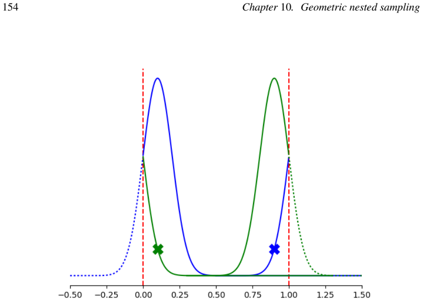
The load-bearing object is the physical cluster model: a spherically symmetric cluster in hydrostatic equilibrium, with dark matter following an NFW profile and gas pressure following a generalised-NFW profile whose slopes are fixed to universal values. Given inputs $M(r_{200})$, $f_{\mathrm{gas}}(r_{200})$, and redshift, the hydrostatic equilibrium equation $dP_g/dr = -\rho_g GM(r)/r^2$ together with the NFW mass integral determines the gas density and pressure normalisation, giving a predicted Comptonisation pattern that is Fourier-transformed into AMI visibilities. The same machinery, with an Einasto dark-matter profile replacing NFW, produces the alternative model tested on cluster A611 and on simulations. For the Planck side, the PowellSnakes detection algorithm supplies the two-dimensional $Y$--$\theta_p$ posteriors that are sliced with a scaling-relation function to obtain the catalogue masses. The geometric nested sampler works by maintaining a set of active points and proposing new points that satisfy the current likelihood constraint using geometric transformations of the parameter domain.

What would settle it

Take the same 54 clusters and measure their masses with weak-lensing shear and X-ray hydrostatic analysis; if the independent masses track Planck's slicing-function values rather than AMI's, the AMI physical model is biased low, while if they track AMI's values, the Planck scaling-relation calibration is biased high. A sharper test is to simulate clusters with a realistic, non-universal pressure profile and analyse them with the fixed-slope physical model: reproducing the observed 37-of-54 offset would pin the discrepancy on the universal-profile assumption.

Watch

Extended reading notes

Core claim

The central claim is that standard Planck mass estimates for the 54-cluster sample are systematically higher than interferometric AMI mass estimates, and that the difference is not fully explained by instrumental noise, CMB contamination, or radio-source environments. The paper reports that AMI $M(r_{500})$ is lower than the PSZ2 slicing-function mass in 37 of 54 clusters and lower than the marginalised PSZ2 mass in 45 of 54; the slicing-function value, which folds in X-ray information, is the closer of the two Planck estimates to the AMI result. Simulations show that when clusters are generated with the same model used in the inference and only instrumental noise is present, 51 of 54 clusters recover the input mass within one standard deviation, but adding confusion noise, primordial CMB, and the actual LA-measured source environments leaves 16 of 54 outside that range, and the recovered-mass distributions become negatively skewed. The thesis therefore attributes the remaining real-data discrepancy to a systematic difference between AMI and Planck data and/or the cluster models, and identifies the fixed 'universal' GNFW pressure profile as a plausible source of model error. A separate contribution is the geometric nested sampler, an adaptation of Metropolis-Hastings nested sampling that exploits the geometry of the parameter domain to satisfy likelihood constraints and is compared with established samplers.

Load-bearing premise

The AMI mass estimates and the Planck comparison both rest on the assumption that every cluster is spherically symmetric, in hydrostatic equilibrium, has a gas mass fraction much less than unity, and follows the universal generalised-NFW pressure profile with fixed slope parameters; if real clusters deviate from that profile, the AMI masses are biased and the apparent Planck-AMI offset is partly a model artefact.

Editorial extensions

If this is right

If the systematic offset is real, cosmological analyses that use Planck PSZ2 masses and the $Y$--$M$ scaling relation should be re-examined, since cluster masses would be overestimated relative to interferometric measurements.
The slicing-function masses, which incorporate X-ray information, agree with AMI better than the marginalised masses, supporting the use of external calibration in Planck mass estimation.
Simulations including confusion noise, CMB, and realistic radio-source environments show negative mass bias, so pipeline validation that omits these components will understate systematic errors.
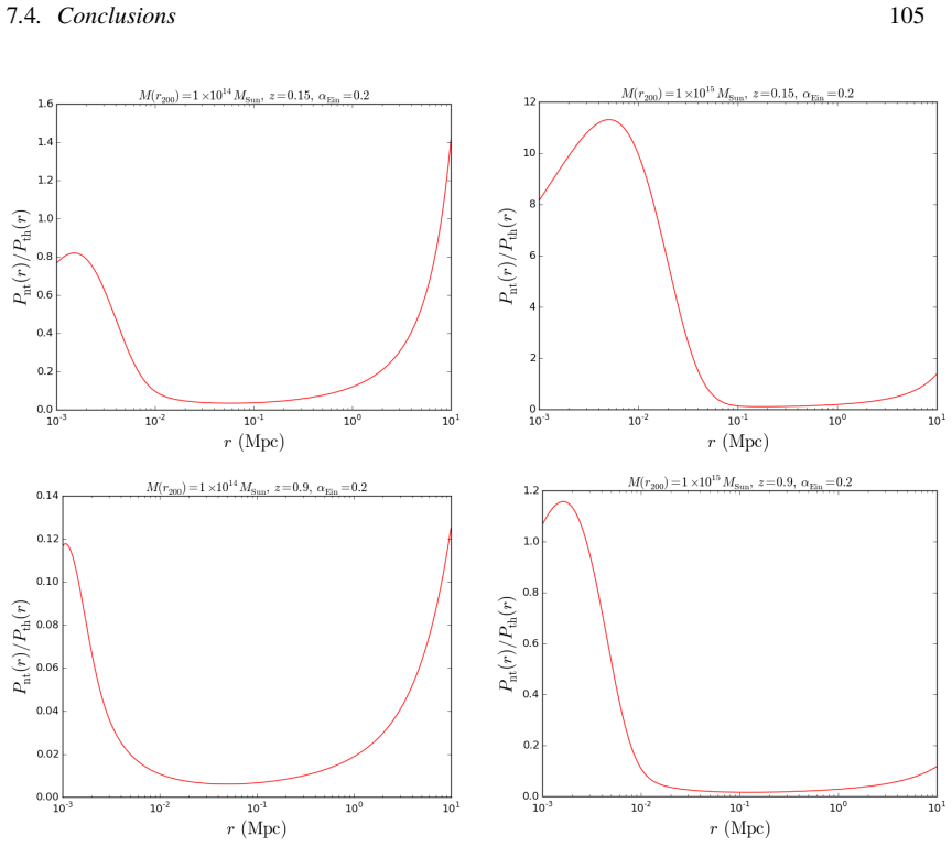
The Einasto dark-matter model recovers input masses better than NFW in 15 of 16 simulations, implying that the assumed dark-matter profile shape contributes to mass-estimate offsets.
The joint AMI-Planck likelihood analysis, while prevented from using hyperparameters by the likelihood-ratio normalisation issue, provides a framework for simultaneous fitting of the two datasets.

Reading between the lines

Editorial extensions of the paper, not claims the author makes directly.

If the offset is mostly model error rather than instrumental difference, then independent mass calibrators such as weak-lensing shear or X-ray hydrostatic masses on the same 54 clusters would be expected to land nearer the AMI values than the Planck slicing-function values; the thesis does not perform this test.
The negative bias seen in the realistic simulations implies that even the AMI masses may be biased low, so the true Planck-minus-AMI offset could be larger than the 37-of-54 and 45-of-54 counts suggest.
Fixing the GNFW slope parameters to universal values is the most consequential assumption; releasing them as free parameters in the same physical model would provide a direct test of whether profile deviations produce the observed offset.
The geometric nested sampler's geometry-based proposals may extend naturally to other problems with correlated or curved parameter spaces, such as gravitational-wave parameter estimation with degenerate masses, though the thesis only demonstrates a single black-hole-merger model.

Share X Bluesky LinkedIn Reddit HN

Signed reviews

No signed human review yet.

Editorial analysis

A structured set of objections, weighed in public.

Desk editor's note, referee report, and a circularity audit.

Desk Editor's Note

read the letter

The thing to know: this is a serious PhD thesis, not a flashy claim. The durable contributions are the AMI mass estimates for 54 Planck clusters, a new Einasto-based physical cluster model, and a geometric nested sampler. The central empirical result—AMI masses come in lower than Planck PSZ2 masses—is probably real, but the thesis cannot fully prove that it reflects a data-level systematic rather than the shared GNFW pressure model.

What it does well: the sample selection is described honestly, with explicit discussion of the biases introduced in cutting from 199 to 54 clusters. The simulation campaign is thoughtfully designed, with four noise/source environments, and the negative skew under realistic conditions is a useful caution. The comparison of physical vs observational models using Earth Mover's distance and evidences is more careful than typical. The Einasto model derivation is clean, and the A611 analysis plus 16 simulations are a reasonable first look. The geometric nested sampler, described but not assessed here, is a plausible original contribution.

Soft spots, in proportion: the simulations in Chapter 3 inject clusters built from the same GNFW profile (with Arnaud slope parameters) used for inference, and the input masses come from the same slicing function used for the PSZ2 masses. So the recovered biases calibrate the pipeline under the model, not the model's realism. The thesis acknowledges this possibility (Sec 2.4.3, citing Perrott et al. 2015) but does not propagate it into the 37/54 and 45/54 comparisons. That is the load-bearing caveat. Second, the Einasto simulation results are odd: Einasto recovers NFW-simulated masses better than NFW in 3 of 4 cases, and only 2 of 16 analyses recover the input mass within 3 sigma. The thesis blames pixelation/binning and underestimated errors, which may be right, but the pattern is concerning enough that the chapter should be read as exploratory, not conclusive. Third, the OM II priors are derived from PM calculations, which makes the OM II vs PM comparison partially circular; the thesis says this, but the evidence ratios in Chapter 4 should be interpreted with that in mind.

Who it's for: cluster cosmologists interested in AMI-Planck calibration, and people working on nested sampling algorithms. It deserves a serious referee—not a desk reject—though the best use would be to extract the published papers and treat the thesis as supporting material.

Referee Report

4 major / 5 minor

Summary. This PhD thesis presents Bayesian inference applied to Sunyaev-Zel'dovich observations of galaxy clusters. The central empirical study compares AMI interferometric mass estimates with two Planck PSZ2/PwS mass estimates for a sample of 54 clusters, finding that AMI masses are lower than the Planck slicing-function masses in 37 of 54 cases and lower than the marginalised Planck masses in 45 of 54 cases. The thesis then uses AMI simulations with Planck-derived input masses to quantify the bias of the AMI pipeline. It further compares a physical cluster model (NFW dark matter plus GNFW gas) with two observational models using parameter estimates, an Earth mover's distance metric, and Bayesian evidences; introduces an Einasto dark-matter variant of the physical model; explores relaxations of the fgas assumption and inclusion of non-thermal pressure; develops a joint AMI-Planck likelihood analysis; and finally presents a new nested-sampling algorithm, the geometric nested sampler, with applications to toy models and gravitational-wave signals.

Significance. If the AMI-Planck mass offset is real, it would have implications for Planck cluster cosmology and for SZ-based mass calibration. The thesis contains substantial and useful work: a carefully selected 54-cluster sample, explicit discussion of selection biases, a large simulation campaign, a new metric-based model comparison, and a new sampling algorithm tested on several problems. The thesis is also unusually candid about its limitations, including the possibility that the universal GNFW pressure profile is not accurate and the fact that some enhanced models are only exploratory. However, the main quantitative claims in Chapters 3 and 5 are not yet fully supported, because the simulations and the Planck mass inputs share the same GNFW model assumptions and because the Einasto simulation conclusions rest on posterior-mean comparisons despite large systematic offsets.

major comments (4)

[§3.7, §3.8 (with §2.4.3 and §3.4.1)] The simulation calibration in §3.7 injects clusters built from the same physical model that is then used for inference: the GNFW pressure profile with slopes fixed to Arnaud et al. (2010), fgas = 0.13, and input masses derived from the PSZ2 slicing function, which itself assumes the same GNFW profile family and Arnaud scaling relations (§3.4.1, Eqs. 3.2–3.5). The measured medians (−0.24 to −0.34 σ in cases 1–4) therefore calibrate the inference pipeline under the assumed model, but do not calibrate the realism of that model. The last bullet of §3.8 is carefully worded ('AMI & Planck data and / or the cluster models'), but the quantitative conclusion that the simulations do not fully accommodate the discrepancy—and the associated 37/54 and 45/54 comparisons in §3.6—still presuppose that the universal GNFW profile is accurate. The thesis itself cites Perrott et al. (2015) in §2.4.3 for the possibility that pressure profiles deviate from the universal profile. This is a genuine calibration loop for the central claim; it should be addressed by adding model-mismatch simulations with perturbed pressure-profile slopes or realistic scatter, or by anchoring masses to X-ray/lensing data, and by reporting how the 37/54 and 45/54 counts change under such perturbations.
[§5.2.2.2 and Table C.1] The Einasto simulation analysis is reported as showing that the Einasto model recovers the input mass better than the NFW model in 15 of 16 cases, but the same results show that only 2 of 16 Einasto analyses recover the input mass within three standard deviations, and that the Einasto model beats NFW even on NFW-generated data in 3 of 4 cases. The thesis attributes the poor recovery to pixelation, u-v binning, and nested-sampling error underestimation (§5.2.2.2). If those error underestimations are present, the posterior-mean comparison is not a valid measure of model performance. The conclusion in §5.3 therefore overstates what the simulations establish: the Einasto model may be more flexible, but the systematic offsets need to be modelled and corrected before one can claim improved mass recovery.
[§4.2.2, §4.3.4.3, §4.4] The comparison between the physical model (PM) and observational model II (OM II) is partially circular because OM II's priors on Ytot and θp are computed from PM calculations (§4.2.2), inheriting PM's assumptions of hydrostatic equilibrium and fgas much less than unity. Consequently the evidence ratios in §4.3.4.3 and the conclusion in §4.4 that PM is preferred over OM II for 43 of 54 clusters are not independent tests of the two models. The thesis acknowledges this in §4.2.2, but the interpretation should be downgraded from model comparison to an internal-consistency check, or OM II should be given priors derived from independent X-ray or Planck data.
[§8.2.2, §8.5–8.6] The joint AMI-Planck analysis is presented as a method for combining independent datasets, but §8.2.2 shows that the likelihood-hyperparameter approach cannot be used with the PwS likelihood ratio, so the analysis is forced to set α1 = α2 = 1. This means the joint likelihood gives equal weight to the two instruments' noise models even when their systematic uncertainties are poorly known; the joint posterior widths and evidence ratios in §8.5–8.6 are therefore optimistic if either likelihood is mis-specified. The text should either implement a properly normalised PwS likelihood or explicitly frame the equal-weight product as a preliminary consistency check rather than the final joint-analysis method.

minor comments (5)

[§2.4.3] The sentence 'For values For values r/rp ≫ 1' contains a duplicated phrase and should be corrected.
[§8.2.2] The text refers to 'MP02' when discussing the toy model of Hobson et al. (2002), but the same method is elsewhere called 'MH02'; the notation should be made consistent.
[§5.1.0.2] The two sets of Arnaud et al. GNFW parameters (a = 1.0620, b = 5.4807, c = 0.3292 and a = 1.0510, b = 5.4905, c = 0.3081) are quoted in the text without a summary table; a small table would reduce the risk of confusion.
[§3.6] Figures 3.6 and 3.7 use row number as the x-axis for clarity, but because row number is monotonic in redshift, the visual impression depends on the cluster ordering; adding redshift ticks or plotting directly against z would improve interpretability.
[§3.8] The first bullet of the conclusions says 'We have made observations' in a single-author thesis; 'I have made observations' would be more consistent with the rest of the text.

Circularity Check

1 steps flagged · score 2.0 of 10

Central AMI-Planck mass comparison is independent of the model loop; only the PM-derived OM II prior creates a self-referential model comparison, and the thesis explicitly acknowledges the closed-loop simulations.

self definitional [Section 4.2.2 (Observational model II); used in the PM vs OM II comparison of Section 4.3.4.3]
"From the z and M(r200) priors of the PM and for fgas(r200) = 0.13, upper and lower bounds on Ytot and θp are calculated using the PM. ... Note that in using the PM calculations to calculate the prior limits, we have made the assumptions underlying the PM that OM I is not subject to (i.e. hydrostatic equilibrium up to radius r200 and fgas is much less than unity up to the same radius)."

OM II is not an independent observational model: its prior support in (Ytot, θp) is computed from the physical model PM and from PM's assumptions. Therefore the later finding that PM and OM II often agree (no conclusive preference in 51 clusters) is partly an artefact of construction: the OM II prior was generated by mapping PM's parameter space through the PM calculations. The PM-vs-OM I comparison is not affected in this way, but the PM-vs-OM II comparison cannot be read as an independent validation of the physical model. The thesis acknowledges the shared assumptions, which limits the severity of the circularity.

full rationale

The thesis's central empirical result is the direct comparison of AMI-derived M(r500) with two PSZ2 mass estimates for the same 54 real clusters (Section 3.6). That comparison does not reduce to a fit: the AMI estimates come from a Bayesian analysis of real interferometric data, and the PSZ2 values are external catalogue entries produced by the Planck PwS pipeline. The conclusion in Section 3.8 is carefully hedged as 'a systematic difference between the AMI & Planck data and / or the cluster models', so it does not claim to have isolated a model-independent offset. The simulations in Section 3.7 do use the same physical model both to generate and to analyse clusters, and the thesis explicitly says 'inferring results from data which was created using the same model used in the inference would be more accurate than results from data taken from two different telescopes, which use different models in their inference.' This is an acknowledged closed-loop self-consistency check, not a hidden prediction passed off as independent. It measures pipeline bias under the assumed model, and the caveat that real pressure profiles may deviate from the universal GNFW form is raised in Section 2.4.3 via Perrott et al. (2015). The only genuine construction-dependent step is the OM II prior in Section 4.2.2, which is derived from the PM and then compared with the PM; this is a partial circularity in a model-comparison chapter, not in the central mass-offset claim. No load-bearing self-citation chain or uniqueness-import argument appears. The paper is substantially self-contained against external Planck catalogue values and external Arnaud et al. (2010) profile parameters, so the circularity score is low.

Assumptions & free parameters 5 free parameters · 8 assumptions · 0 invented entities

The central mass estimates depend on several externally fitted relations: the GNFW pressure profile slopes from Arnaud et al. (2010), the concentration-mass relations from Neto et al. (2007), Wechsler et al. (2001) and Dutton and Macciò (2014), the non-thermal pressure coefficient from Martizzi and Agrusa (2016), and the Planck scaling relations used for PSZ2 masses. These are not fitted in this thesis but are numbers fitted to data elsewhere. The model also relies on domain assumptions of spherical symmetry, hydrostatic equilibrium, and ideal gas behaviour. No new physical entities are introduced; the geometric nested sampler is a computational algorithm, not an entity.

free parameters (5)

GNFW pressure slope parameters (a, b, c) and c500 = a=1.0620, b=5.4807, c=0.3292, c500=1.156 (Ch 2-4); a=1.0510, b=5.4905, c=0.3081, c500=1.177 (Ch 5)
Universal values from Arnaud et al. (2010) used in computing pressure profiles and masses; the thesis does not fit them.
NFW concentration-mass relation parameters = c200 = 5.26/(1+z) (M/1e14 h^-1 Msun)^-0.1
Fitted to N-body simulations in Neto et al. (2007) and Wechsler et al. (2001); used to set scale radius and hence mass estimates.
Einasto concentration-mass relation parameters j(z), k(z) = j(z)=0.459+0.518 exp(-0.49 z^1.303), k(z)=-0.13+0.029 z
Fitted in Dutton and Macciò (2014); used for the Einasto model in Chapter 5.
Non-thermal pressure coefficient beta = 5.658e-36 Mpc^2 s^-2
Fitted to simulations in Martizzi and Agrusa (2016); used in Chapter 7 to compute Pnt/Pth ratios.
Planck Y-M and theta-M scaling relations = Y-M slope 1.79, normalization 10^-0.19, bias (1-b)=0.80
Fitted to X-ray/SZ samples in Planck Collaboration et al. (2014); used to convert PwS Y values to PSZ2 masses.

assumptions (8)

domain assumption Clusters are spherically symmetric
Section 2.4.1, allows scalar radius parameterisation.
domain assumption Hydrostatic equilibrium up to r200
Section 2.4.1, equation 2.30.
domain assumption Gas mass fraction is much less than unity up to r200, so M is approximately Mdm
Section 2.4.1, used to derive mass and pressure normalisation.
domain assumption ICM behaves as an ideal gas
Section 2.4.1, used to relate pressure and temperature.
domain assumption GNFW profile describes the electron pressure
Section 2.4.3, equation 2.21, based on Nagai et al. (2007) and Arnaud et al. (2010).
domain assumption NFW/Einasto profiles describe dark matter density
Sections 2.4.2 and 5.1, equations 2.19 and 5.1.
standard math AMI visibilities have Gaussian likelihood
Section 2.8, equations 2.49-2.52, following Hobson and Maisinger (2002).
domain assumption AMI and Planck data are independent in the joint analysis
Section 8.1.3, equation 8.2.

how reviews work

0 comments

Cite this review

Pith. "Pith review of Physical modelling of galaxy clusters and Bayesian inference in astrophysics." pith.science (2026). https://pith.science/paper/IYCZVY5O

@misc{pith2026190900029,
  author       = {Pith},
  title        = {Pith review of: Physical modelling of galaxy clusters and Bayesian inference in astrophysics},
  year         = {2026},
  howpublished = {\url{https://pith.science/paper/IYCZVY5O}},
  note         = {Machine review of arXiv:1909.00029}
}

read the original abstract

I compare the mass values obtained with data taken from the Arcminute Microkelvin Imager (AMI) radio interferometer system and from the Planck satellite. The former of these uses a Bayesian analysis pipeline that parameterises a cluster in terms of its physical quantities, and models the dark matter \& baryonic components of a cluster using Navarro-Frenk-White (NFW) and generalised-NFW profiles respectively. I also analyse simulated AMI data with input values based on PwS mass estimates. I then compare three cluster models using AMI data for the 54 cluster sample. The two observational models considered only model the gas content of the cluster. To compare the physical and observational models I consider their posterior parameter estimates, including the calculation of a metric defined between two probability distributions. The models' fit to the cluster data is evaluated by looking at the Bayesian evidence values. Improvements to the physical modelling of galaxy clusters are then considered, either by relaxing some of the assumptions underlying the physical model, or by introducing a new profile for the dark matter component of clusters. The final part of the cluster analysis work focuses on Bayesian analysis using a joint likelihood function of data from both AMI and the Planck satellite simultaneously. Finally, a new Bayesian inference algorithm based on nested sampling is presented. The algorithm, named the "geometric nested sampler", is an adaption of the Metropolis-Hastings nested sampler and makes use of the geometrical interpretation of sets of parameters to sample from their domains efficiently. The geometric nested sampler is tested on several toy models as well as a model representing the emission of gravitational waves from binary black hole mergers.

Figures

Figures reproduced from arXiv: 1909.00029 by the authors.

**Figure 1.1.** Radiation intensity as a function of frequency. Note the dashed line represents the incident radiation, whilst the solid line represents the energy-boosted inverse Compton scattered radiation. Taken from Carlstrom et al. (2002) [PITH_FULL_IMAGE:figures/full_fig_p015_1_1.png] view at source ↗

**Figure 2.1.** Simple east-west single baseline interferometer tracking a patch of sky containing a single radio-source. For a baseline b and a source at angle θ from the vertical axis, the wavefront has to travel an additional distance b sin θ to the further antenna. Image taken from Zaroubi (2013). observed and k is the corresponding wavenumber. The ωt-dependent parts are removed and the correlator multiplies the remaining compo… view at source ↗

**Figure 2.2.** Spectral index distribution adapted from Waldram et al. (2007) from the 9C survey of radio-sources. π(Srs,0) = N (Srs,0, LA, σrs,0). The spectral index αrs was modelled using the empirical distribution determined in Waldram et al. (2007): π(αrs) = W(αrs) and is shown in [PITH_FULL_IMAGE:figures/full_fig_p036_2_2.png] view at source ↗

Figures from the paper (72 more)

**Figure 3.1.** Figure 3.1: Example of the posterior slicing methodology for cluster PSZ2G228.16+75.20. The black solid line represents the ‘ridge’ (i.e. the most probable value of Y(5r500) for each θp) of the posterior. The upper dashed curve represents the upper boundaries of the 68% maximum…

**Figure 3.2.** Figure 3.2: Posterior distributions derived from AMI data for the sampling parameters: M(r200); fgas(r200); xc & yc. The contoured maps show the two-dimensional posteriors for the different pairs of parameters. The contours represent the 95% and 68% mean confidence intervals, wi…

**Figure 3.3.** Figure 3.3: (a) Unsubtracted map produced from AMI observation. Contours are plotted at ±(2, 3, 4, ..., 10)× the r.m.s. noise level, and dashed contours are negative. (b) Source subtracted map produced from AMI observation. The denotes the McAdam-determined centre of the cluster…

**Figure 3.4.** Figure 3.4: Subtracted map of cluster with ill-defined centre. The cluster is clearly offset from the observation pointing centre (middle of the map), and the lobes to the bottom and the top left of the cluster cause the centre position to be ambiguous. and Planck data is 54. It…

**Figure 3.5.** Figure 3.5: Plot of M(r200) derived from AMI data using physical modelling vs redshift for the sample of 54 clusters. have discrepancies larger than three combined standard deviations. Three of these clusters are at relatively low redshift (≤ 0.25), whilst one is at z = 0.43. It…

**Figure 3.6.** Figure 3.6: Plot of M(r500) vs row number of Table A.1 for three different cases: the value derived from AMI data using the physical model, MAMI(r500); the value derived from Planck data using the marginalised value for Y(5r500), MPl, marg(r500) and the value derived from Planck…

**Figure 3.7.** Figure 3.7: Plot of M(r500) ratios vs row number of Table A.1 for three different cases: MAMI(r500)/MPl, marg(r500); MAMI(r500)/MPl, slice(r500) and MPl, marg(r500)/MPl, slice(r500). The points with square markers correspond to clusters whose redshifts were measured spectroscopi…

**Figure 3.8.** Figure 3.8: Unsubtracted map produced from simulated AMI data of cluster PSZ2G044.20+48.66, including instrumental noise [PITH_FULL_IMAGE:figures/full_fig_p055_3_8.png]

**Figure 3.9.** Figure 3.9: Normalised histogram of the differences between the input and output masses of the AMI simulations including the cluster and instrumental noise only, in units of standard deviations of the output mass. at low redshift (z < 0.2). This suggests that the confusion and C…

**Figure 3.10.** Figure 3.10: Unsubtracted map produced from simulated AMI data of cluster PSZ2G044.20+48.66, including instrumental, confusion and CMB noise. including a canonical source environment and background noise. The mass estimate derived from the Bayesian analysis of this cluster is 0.…

**Figure 3.11.** Figure 3.11: Normalised histogram of the differences between the input and output masses of the AMI simulations, in units of standard deviations of the output mass. This is the case for instrumental, confusion and CMB noise contributions. was just a coincidence. 3.7.4 Simulation…

**Figure 3.12.** Figure 3.12: Unsubtracted map produced from simulated AMI data of cluster PSZ2G044.20+48.66, including a canonical radio-source environment as well as instrumental, confusion and CMB noise [PITH_FULL_IMAGE:figures/full_fig_p059_3_12.png]

**Figure 3.13.** Figure 3.13: Normalised histogram of the differences between the input and output masses of the AMI simulations, in units of standard deviations of the output mass. This is the case for a canonical radio-source environment as well instrumental, confusion and CMB noise contributi…

**Figure 3.14.** Figure 3.14: (a) Unsubtracted map produced from real AMI data of cluster PSZ2G044.20+48.66. (b) Unsubtracted map produced from simulated AMI data of PSZ2G044.20+48.66, including the real source environment (as measured by the LA) as well as instrumental, confusion and CMB noise.…

**Figure 3.15.** Figure 3.15: Normalised histogram of the differences between the input and output masses of the AMI simulations, in units of standard deviations of the output mass. This is the case for the real radio-source environment as measured by the LA, with instrumental, confusion and CMB…

**Figure 4.1.** Figure 4.1: Plot of Y(r500) obtained from AMI data using the physical and observational models vs row number of Table B.1. The points with circular markers correspond to clusters whose redshifts were measured photometrically as opposed to spectroscopically. For clarity purposes…

**Figure 4.2.** Figure 4.2: Plot of Y(r500) ratio vs row number of Table B.1 for three different cases: YPM(r500)/YOM I(r500); YPM(r500)/YOM II(r500) and YOM I(r500)/YOM II(r500). The points with square markers correspond to clusters whose redshifts were measured spectroscopically, and the circ…

**Figure 4.3.** Figure 4.3: (a) Highest dEMD value Y(r500) − θ500 posteriors for cluster PSZ2G044.20+48.66 at z = 0.0894. (b) Lowest dEMD value Y(r500) − θ500 posteriors for cluster PSZ2G132.47-17.27 at z = 0.341. For both triangle plots, the top graph shows the marginalised θ500 posteriors fo…

**Figure 4.4.** Figure 4.4: Earth Mover’s distance calculated between Y(r500) − θ500 posteriors for PM and OM II, versus z for the 54 clusters. The crosses indicate the point– they are not error bars. "more data are needed to come to a meaningful conclusion". (see [PITH_FULL_IMAGE:figures/full…

**Figure 4.5.** Figure 4.5: (a) Lowest z (= 0.0894) prior parameter space for Y(r500) − θ500 using the PM. (b) Highest z (= 0.83) prior parameter space for Y(r500) − θ500 for the PM and OM II. Note the scales on the axes are different for each plot, and the green vertical lines represent the me…

**Figure 4.6.** Figure 4.6: Two-dimensional prior probability distribution of Y(r500) and θ500 for OM I, which is based on Planck data as detailed in Section 4.2.1. 4.3.4.3 Physical model and observational model II Comparison of PM and OM II, the models which incorporate redshift information in…

**Figure 5.1.** Figure 5.1: Logarithmic dark matter density profiles as a function of log cluster radius using NFW and Einasto models. Three values of the Einasto profile are used: 0.05, 0.2, and 2.0. The additional input parameters used to generate these profiles are: z = 0.15, M(r200) = 1 × 1…

**Figure 5.2.** Figure 5.2: Dark matter mass profiles as a function of log cluster radius using NFW and Einasto models. Values of αEin = 0.05, 0.2, and 2.0 are used as inputs. Top row has z = 0.15, bottom row has z = 0.9. Left column has M(r200) = 1 × 1014MSun, right column has M(r200) = 1 × 10…

**Figure 5.3.** Figure 5.3: Logarithmic gas density profiles as a function of log cluster radius using NFW and Einasto models. Values of αEin = 0.05, 0.2, and 2.0 are used as inputs. Top row has z = 0.15, bottom row has z = 0.9. Left column has M(r200) = 1 × 1014MSun, right column has M(r200) =…

**Figure 5.4.** Figure 5.4: Gas mass profiles as a function of log cluster radius using NFW and Einasto models. Values of αEin = 0.05, 0.2, and 2.0 are used as inputs. Top row has z = 0.15, bottom row has z = 0.9. Left column has M(r200) = 1 × 1014MSun, right column has M(r200) = 1 × 1015MSun. …

**Figure 5.5.** Figure 5.5: Gas temperature profiles as a function of log cluster radius using NFW and Einasto models. Values of αEin = 0.05, 0.2, and 2.0 are used as inputs. Top row has z = 0.15, bottom row has z = 0.9. Left column has M(r200) = 1 × 1014MSun, right column has M(r200) = 1 × 101…

**Figure 5.6.** Figure 5.6: Marginalised posterior distributions of physical model input parameters for the NFW and αEin = 2.0 models applied to real A611 data. The contour plots are the two dimensional marginalised plots of the parameters named in the corresponding row / column. The line plots…

**Figure 5.7.** Figure 5.7: Posterior distributions for cluster simulated with αEin = 2.0, M(r200) = 1 × 1015MSun and z = 0.9, modelled with: (a) Einasto dark matter profile, and (b) NFW dark matter profile. underestimate in the associated errors. Furthermore, the fact that the Einasto model re…

**Figure 5.8.** Figure 5.8: Posterior distributions for cluster simulated with αEin = 2.0, M(r200) = 1 × 1014MSun and z = 0.9, modelled with: (a) Einasto dark matter profile, and (b) NFW dark matter profile. model (ln (ZEin/ZNFW) ≥ 5). In two of these cases (αEin = 0.2 with M(r200) = 1×1015MSun…

**Figure 5.9.** Figure 5.9: Posterior distributions of Einasto model input parameters for: (a) αEin = 2.0, M(r200) = 1 × 1014MSun and z = 0.15 simulated cluster, and (b) αEin = 2.0, M(r200) = 1 × 1014MSun and z = 0.9 simulated cluster. 2.39 ± 0.40), but looking at the distributions they are not…

**Figure 6.1.** Figure 6.1: Mass profiles of cluster with input parameters given in titles. PM I (NFW dark matter profile, M(r) ≈ Mdm(r) approximation) and PMT I (NFW dark matter profile, M(r) = Mdm(r) + Mg(r)) are shown in the top left graph by black and red curves respectively. The other thre…

**Figure 6.2.** Figure 6.2: Mass profiles of cluster with input parameters given in title, for models given in [PITH_FULL_IMAGE:figures/full_fig_p102_6_2.png]

**Figure 6.3.** Figure 6.3: Mass profiles of cluster with input parameters given in title, for models given in [PITH_FULL_IMAGE:figures/full_fig_p103_6_3.png]

**Figure 6.4.** Figure 6.4: Mass profiles of cluster with input parameters given in title, for models given in [PITH_FULL_IMAGE:figures/full_fig_p104_6_4.png]

**Figure 7.1.** Figure 7.1: ρg(r) profiles for PM I and PMN I. Each graph features both profiles for one of the four different input parameter sets. Top row has z = 0.15, bottom row has z = 0.9. Left column has M(r200) = 1 × 1014MSun, right column has M(r200) = 1 × 1015MSun described in Section…

**Figure 7.2.** Figure 7.2: ρg(r) profiles for PM II and PMN II with αEin = 0.05. Graphs are laid out as described in [PITH_FULL_IMAGE:figures/full_fig_p111_7_2.png]

**Figure 7.3.** Figure 7.3: ρg(r) profiles for PM II and PMN II with αEin = 0.2. Graphs are laid out as described in [PITH_FULL_IMAGE:figures/full_fig_p112_7_3.png]

**Figure 7.4.** Figure 7.4: ρg(r) profiles for PM II and PMN II with αEin = 2. Graphs are laid out as described in [PITH_FULL_IMAGE:figures/full_fig_p113_7_4.png]

**Figure 7.5.** Figure 7.5: Ratio of Pnt to Pth profiles for PM I and PMN I. Each graph features both profiles for one of the four different input parameter sets. Top row has z = 0.15, bottom row has z = 0.9. Left column has M(r200) = 1 × 1014MSun, right column has M(r200) = 1 × 1015MSun they d…

**Figure 7.6.** Figure 7.6: Ratio of Pnt to Pth profiles for PM II and PMN II with αEin = 0.05. Graphs are laid out as described in [PITH_FULL_IMAGE:figures/full_fig_p115_7_6.png]

**Figure 7.7.** Figure 7.7: Ratio of Pnt to Pth profiles for PM II and PMN II with αEin = 0.2. Graphs are laid out as described in [PITH_FULL_IMAGE:figures/full_fig_p117_7_7.png]

**Figure 7.8.** Figure 7.8: Ratio of Pnt to Pth profiles for PM II and PMN II with αEin = 2. Graphs are laid out as described in [PITH_FULL_IMAGE:figures/full_fig_p118_7_8.png]

**Figure 8.1.** Figure 8.1: Top: Two-dimensional posterior distribution obtained from application of likelihood hyperparameter method on toy model considered in Section 6.1 of MP02. m and c are the gradient and intercept parameters of the toy model respectively. These results were obtained usin…

**Figure 8.2.** Figure 8.2: Two-dimensional marginalised xc − yc and Ytot −θp posterior distributions for a high SNR (see Section 8.5.1) cluster simulation generated using OM III. The red contours correspond to the posterior distribution associated with the AMI and Planck datasets which had dif…

**Figure 8.3.** Figure 8.3: Two-dimensional marginalised xc − yc and Ytot −θp posterior distributions for the 10 OM III low SNR cluster simulations obtained from: AMI data (top row), Planck data (middle row), and AMI and Planck data combined (bottom row). The contours in each plot represent the…

**Figure 8.4.** Figure 8.4: Two-dimensional marginalised xc − yc and Ytot −θp posterior distributions for the 10 OM III high SNR cluster simulations. The Figure layout is as described in [PITH_FULL_IMAGE:figures/full_fig_p132_8_4.png]

**Figure 8.5.** Figure 8.5 [PITH_FULL_IMAGE:figures/full_fig_p134_8_5.png]

**Figure 8.6.** Figure 8.6: Two-dimensional marginalised posterior distributions for six OM III high SNR cluster simulations where a and b were allowed to vary in the analysis. The plot layout is as described in [PITH_FULL_IMAGE:figures/full_fig_p135_8_6.png]

**Figure 8.7.** Figure 8.7: One-dimensional marginalised posterior distributions for the 10 PM I low SNR cluster simulations obtained from: AMI data (top row), Planck data (middle row), and AMI and Planck data combined (bottom row). The black vertical lines indicate the values input when genera…

**Figure 8.8.** Figure 8.8: One-dimensional marginalised posterior distributions for the 10 PM I high SNR cluster simulations. The plots are laid out as described in [PITH_FULL_IMAGE:figures/full_fig_p138_8_8.png]

**Figure 8.9.** Figure 8.9: One-dimensional marginalised posterior distributions for the 10 PM II high SNR cluster simulations obtained by marginalising over αEin. The plots are laid out as described in [PITH_FULL_IMAGE:figures/full_fig_p140_8_9.png]

**Figure 8.10.** Figure 8.10: Marginalised posterior distributions obtained from joint AMI-Planck analysis of cluster PSZ2G063.80+11.42, using PM I. The dashed line plots are fully marginalised posterior distributions, while the contour plots are two-dimensional marginalised distributions. The …

**Figure 8.12.** Figure 8.12 [PITH_FULL_IMAGE:figures/full_fig_p143_8_12.png]

**Figure 9.1.** Figure 9.1: Left: Illustrating inverse transform sampling for a one-dimensional distribution P(θ). Once a value for ui is obtained, one draws a horizontal line from (0, u) until it intersects with F (θ) (black dotted line). The value of θ at the point of intersection is the poi…

**Figure 9.2.** Figure 9.2: Left plot: Five iso-likelihood contours of a two-dimensional, multi-modal likelihood L(θ1, θ2). Each contour encloses some fraction of the prior X, with the colourscale indicating the value of X (darkest: smallest X). Right: Corresponding L as a function of X plot (n…

**Figure 9.3.** Figure 9.3: Plots of L(X) and L(X)X for typical likelihood functions. The area under the L(X) curve corresponds to Z. The height of the curve L(X)X, gives an indication of the contribution to Z for a small fractional change in X. After a number of nested sampling iterations, thi…

**Figure 9.4.** Figure 9.4: Illustration of approximationg a one-dimensional posterior function P(θ) using a histogram or KDE. P(θ) is a Gaussian mixture model (parameterised in terms of means and standard deviations): P(θ) = 0.8 × N (−1, 1) + 0.2 × N (1, 0.3). The samples S = {(θ1, P1), ..., (…

**Figure 10.1.** Figure 10.1: ‘Vanilla’ non-wrapped trial distribution. The blue curve represents a Gaussian ‘vanilla’ trial distribution q(θ 0 |θ) with starting point θ = 0.1, and sampled trial point θ 0 = −0.1 shown by the blue cross. The support of π is indicated by the red dashed lines ([0, …

**Figure 10.2.** Figure 10.2: Wrapped trial distributions. The solid blue curve represents a Gaussian trial distribution q(θ 0 |θ) as in previous Figure, but now incorporating the wrapping methodology. As a result of the wrapping, θ 0 (blue cross) is at 0.9, and so won’t be automatically rejecte…

**Figure 10.3.** Figure 10.3: von Mises distribution with domain [−π, π], centred on π. The peak wraps around at edges of domain, so that it appears as two half peaks on a linear space. of modes, to ensure both half peaks are sampled adequately without one cluster ‘dying out’. Furthermore, the t…

**Figure 10.4.** Figure 10.4: Sampling points on the surface of a sphere in Cartesian coordinates. The three-dimensional trial distribution is centred at the point (xl , yl , zl), which corresponds to (φl , θl). The point (x 0 , y 0 , z 0 ) sampled from q in general will not lie on the surface o…

**Figure 10.5.** Figure 10.5: Sampling points on the perimeter of a circle in Cartesian coordinates. The two-dimensional trial distribution is centred at the point(xl , yl), which corresponds to φl . The point (x 0 , y 0 ) sampled from q in general will not lie on the perimeter of the circle, ho…

**Figure 10.6.** Figure 10.6: Sampling points on the surface of a torus with major and minor radii R and r in Cartesian coordinates. R corresponds to the distance from the centre of the torus (centre of the whitespace in the middle of the grey tube) to the centre of the cross section (depicted a…

**Figure 10.7.** Figure 10.7: Torus cross section at φ = φp and φ = φp + π in x–z plane. If the sampled point lies in the half-plane (shaded blue) defined by φ = φp, it will be projected onto the circle in this half-plane, otherwise it will be projected onto the circle in the φ = φp + π half-pla…

**Figure 10.8.** Figure 10.8: Posterior distributions of the circular toy model defined in Section 10.4.1. The black curve corresponds to samples obtained from the analytical expression for P(φ) evaluated over a range of φ values. The blue, red and green curves correspond to the samples obtained…

**Figure 10.9.** Figure 10.9: Posterior distributions of the circular toy model with the number of livepoints set to 500. The colour coding of the plot is as described in [PITH_FULL_IMAGE:figures/full_fig_p178_10_9.png]

**Figure 10.10.** Figure 10.10: Posterior distributions of the toroidal toy model defined in Section 10.4.2, with the number of livepoints set to 50. The colour coding is as described in [PITH_FULL_IMAGE:figures/full_fig_p180_10_10.png]

**Figure 10.11.** Figure 10.11: Posterior distributions of toroidal toy model with the number of livepoints set to 500. The colour coding and layout of the plots is as explained in [PITH_FULL_IMAGE:figures/full_fig_p181_10_11.png]

**Figure 10.12.** Figure 10.12: Posterior distributions of the spherical toy model with the number of livepoints set to 50. The colour coding and layout of the plots is as explained in [PITH_FULL_IMAGE:figures/full_fig_p182_10_12.png]

**Figure 10.13.** Figure 10.13: Posterior distributions of the spherical toy model with the number of livepoints set to 500. The colour coding and layout of the plots is as explained in [PITH_FULL_IMAGE:figures/full_fig_p183_10_13.png]

**Figure 10.14.** Figure 10.14: Marginalised one- and two-dimensional posterior distributions for the five angular parameters, φc, φ, θ, p, and i. The black curves are the results from the 2000 livepoint MN run. The blue and red curves are plotted using the samples of the MG and MN algorithms res…

**Figure 10.15.** Figure 10.15: Same plot as [PITH_FULL_IMAGE:figures/full_fig_p189_10_15.png]

Discussion (0). Continue with ORCID to comment.

Reference graph

Works this paper leans on

46 extracted references · 42 canonical work pages

[1]

Chevallier,M.,Polarski,D.2001.AcceleratingUniverseswithScalingDarkMatter.International Journal of Modern Physics D 10,

work page 2001
[3]

Monthly Notices of the Royal Astronomical Society 279,

Haehnelt,M.G.,Tegmark,M.1996.UsingtheKinematicSunyaev-Zeldovicheﬀecttodetermine the peculiar velocities of clusters of galaxies.. Monthly Notices of the Royal Astronomical Society 279,

work page 1996
[10]

The Astrophysical Journal 650,

Kravtsov,A.V.,Vikhlinin,A.,Nagai,D.2006.ANewRobustLow-ScatterX-RayMassIndicator for Clusters of Galaxies. The Astrophysical Journal 650,

work page 2006
[12]

Battaglia, N., Bond, J.R., Pfrommer, C., Sievers, J.L.2012.OntheClusterPhysicsofSunyaev- Zel’dovich and X-Ray Surveys. I. The Inﬂuence of Feedback, Non-thermal Pressure, and Cluster Shapes on Y-M Scaling Relations. The Astrophysical Journal 758,

work page 2012
[13]

Why does the Metropolis-Hastings procedure satisfy the detailed balance criterion?

208 References Hauser K. 2013 "Why does the Metropolis-Hastings procedure satisfy the detailed balance criterion?" URL: http://people.duke.edu/~kh269/teaching/notes/ MetropolisExplanation.pdf Herranz,D.,and6colleagues2002.FilteringtechniquesforthedetectionofSunyaev-Zel’dovich clusters <br/> in multifrequency maps. Monthly Notices of the Royal Astron...

work page 2013
[17]

Olamaie, M., Hobson, M

Nyquist,H.1928.ThermalAgitationofElectricChargeinConductors.PhysicalReview32,110. Olamaie, M., Hobson, M. P., Grainge, K. J. B

work page 1928
[18]

KompaneetsA.S. 1957 Theestablishmentofthermalequilibriumbetweenquantaandelectrons Soviet Physics JETP, 4, 730 Korngut,P.M.,and8colleagues2011.MUSTANGHighAngularResolutionSunyaev-Zel’dovich Eﬀect Imaging of Substructure in Four Galaxy Clusters. The Astrophysical Journal 734,

work page 1957
[19]

Monthly Notices of the Royal Astronomical Society 335,

Hobson,M.P.,Bridle,S.L.,Lahav,O.2002.Combiningcosmologicaldatasets: hyperparameters and Bayesian evidence. Monthly Notices of the Royal Astronomical Society 335,

work page 2002

Show all 46 references

[20]

Monthly Notices of the Royal Astronomical Society 489, 3135, DOI:https://doi.org/10.1093/mnras/stz2341

Physical modelling of galaxy References 209 cluster Sunyaev-Zel’dovich data using Einasto dark matter proﬁles. Monthly Notices of the Royal Astronomical Society 489, 3135, DOI:https://doi.org/10.1093/mnras/stz2341. Javid, K., and 7 colleagues

doi
[21]

Monthly Notices of the Royal Astronomical Society 483, 3529, DOI:https://doi

Physical modelling of galaxy clusters detected by the Planck satellite. Monthly Notices of the Royal Astronomical Society 483, 3529, DOI:https://doi. org/10.1093/mnras/sty3115. Javid,K.Geometricnestedsampling: samplingfromdistributionsdeﬁnedonnon-trivialgeomet- ries. Journal o...

doi
[30]

The Astrophysical Journal 731,

The Atacama Cosmology Telescope: Extragalactic Sources at 148 GHz in the 2008 Survey. The Astrophysical Journal 731,

2008
[33]

Navarro,J.F.,Frenk,C.S.,White,S.D.M.1995.SimulationsofX-rayclusters.MonthlyNotices of the Royal Astronomical Society 275,

Nagai,D.,Lau,E.T.2011.GasClumpingintheOutskirtsof ΛCDMClusters.TheAstrophysical Journal 731, L10. Navarro,J.F.,Frenk,C.S.,White,S.D.M.1995.SimulationsofX-rayclusters.MonthlyNotices of the Royal Astronomical Society 275,

2011
[36]

Monthly Notices of the Royal Astronomical Society 486, 2116, DOI:https://doi

Sunyaev-Zel’dovich proﬁle ﬁtting with joint AMI-Planck analysis. Monthly Notices of the Royal Astronomical Society 486, 2116, DOI:https://doi. org/10.1093/mnras/stz826. Petrov,L.,Kovalev,Y.Y.,Fomalont,E.B.,Gordon,D.2008.TheSixthVLBACalibratorSurvey: References 213 VCS6. The As...

2008 doi
[41]

Journal of Cosmology and Astro-Particle Physics 2016,

Comparison of weak lensing by NFW and Einasto halos and systematic errors. Journal of Cosmology and Astro-Particle Physics 2016,

2016
[42]

arXiv e- prints arXiv:1101.5590

Sunyaev-Zel’dovich observations of LoCuSS clusters with the Arcminute Microkelvin Imager: high X-ray luminosity sample. arXiv e- prints arXiv:1101.5590. Silk, J

arXiv
[44]

Journal of Cosmology and Astro- Particle Physics 2006,

Seljak,U.,Slosar,A.,McDonald,P.2006.CosmologicalparametersfromcombiningtheLyman- α forest with CMB, galaxy clustering and SN constraints. Journal of Cosmology and Astro- Particle Physics 2006,

2006
[45]

VizieR Online Data Catalog J/MNRAS/379/1442

VizieR Online Data Catalog: Multifrequency observations of 9C sources (Waldram+, 2007). VizieR Online Data Catalog J/MNRAS/379/1442. Watson,R.A.,and25colleagues2003.FirstresultsfromtheVerySmallArray-I.Observational methods. Monthly Notices of the Royal Astronomical Society 341,

2007
[46]

arXiv e-prints astro-ph/0111069

Concentrations and Assembly Histories of Dark Matter Halos. arXiv e-prints astro-ph/0111069. Weisskopf, M. C., Brinkman, B., Canizares, C., Garmire, G., Murray, S., Van Speybroeck, L. P

arXiv
[97]

Living Reviews in Relativity 17,

Blanchet, L.2014.GravitationalRadiationfromPost-NewtonianSourcesandInspirallingCom- pact Binaries. Living Reviews in Relativity 17,

2014
[245]

Monthly Notices of the References 207 Royal Astronomical Society 395,

George,M.R.,Fabian,A.C.,Sanders,J.S.,Young,A.J.,Russell,H.R.2009.X-rayobservations of the galaxy cluster PKS0745-191: to the virial radius, and beyond. Monthly Notices of the References 207 Royal Astronomical Society 395,

2009
[256]

Astronomy and Computing 5,

Ma,Y.-Z.,Berndsen,A.2014.Howtocombinecorrelateddatasets-ABayesianhyperparameter matrix method. Astronomy and Computing 5,

2014
[449]

Astrophysics Source Code Library ascl:1109.006

Feroz,F.,Hobson,M.P.,Bridges,M.2011.MultiNest: EﬃcientandRobustBayesianInference. Astrophysics Source Code Library ascl:1109.006. Feroz, F., Hobson, M. P., Bridges, M

2011
[539]

Monthly Notices of the Royal Astronomical Society 450,

Rozo,E.,Rykoﬀ,E.S.,Bartlett,J.G.,Melin,J.-B.2015.redMaPPer-III.Adetailedcomparison of the Planck 2013 and SDSS DR8 redMaPPer cluster catalogues. Monthly Notices of the Royal Astronomical Society 450,

2015
[569]

Hu, W., Kravtsov, A

Hoshino, A., and 16 colleagues 2010.X-Ray Temperature and MassMeasurements to the Virial RadiusofAbell1413withSuzaku.PublicationsoftheAstronomicalSocietyofJapan62,371. Hu, W., Kravtsov, A. V

2010
[575]

International Journal of Modern Physics D 23, 1430007-98

Brunetti,G.,Jones,T.W.2014.CosmicRaysinGalaxyClustersandTheirNonthermalEmission. International Journal of Modern Physics D 23, 1430007-98. References 205 Carlstrom, J. E., Holder, G. P., Reese, E. D

2014
[580]

Eﬀects on the Sunyaev-Zel’dovich eﬀect and the X-ray emission

Pfrommer,C.,Enßlin,T.A.,Springel,V.,Jubelgas,M.,Dolag,K.2007.Simulatingcosmicrays in clusters of galaxies - I. Eﬀects on the Sunyaev-Zel’dovich eﬀect and the X-ray emission. Monthly Notices of the Royal Astronomical Society 378,

2007
[594]

The Astrophysical Journal 668,

Nagai,D.,Kravtsov,A.V.,Vikhlinin,A.2007.EﬀectsofGalaxyFormationonThermodynamics of the Intracluster Medium. The Astrophysical Journal 668,

2007
[611]

X-ray and strong lensing analyses

II. X-ray and strong lensing analyses. Astronomy and Astrophysics 528, A73. Dutton,A.A.,Macciò,A.V.2014.ColddarkmatterhaloesinthePlanckera: evolutionofstruc- tural parameters for Einasto and NFW proﬁles. Monthly Notices of the Royal Astronomical Society 441,

2014
[643]

Carvalho,P.,Rocha,G.,Hobson,M.P.2009.AfastBayesianapproachtodiscreteobjectdetection inastronomicaldatasets-PowellSnakesI.MonthlyNoticesoftheRoyalAstronomicalSociety 393,

2009
[657]

Space Science Reviews 177,

Giodini,S.,Lovisari,L.,Pointecouteau,E.,Ettori,S.,Reiprich,T.H.,Hoekstra,H.2013.Scaling Relations for Galaxy Clusters: Properties and Evolution. Space Science Reviews 177,

2013
[702]

The Astrophysical Journal 502,

Itoh,N.,Kohyama,Y.,Nozawa,S.1998.RelativisticCorrectionstotheSunyaev-ZeldovichEﬀect for Clusters of Galaxies. The Astrophysical Journal 502,

1998
[1057]

Monthly Notices of the Royal Astronomical Society 475, 5677, DOI:https://doi

Hickish,J.,and20colleagues2018.AdigitalcorrelatorupgradefortheArcminuteMicroKelvin Imager. Monthly Notices of the Royal Astronomical Society 475, 5677, DOI:https://doi. org/10.1093/mnras/sty074. Higson, E., Handley, W., Hobson, M., Lasenby, A

doi
[1450]

Nozawa,S.,Itoh,N.,Kohyama,Y.1998.RelativisticCorrectionstotheSunyaev-ZeldovichEﬀect for Clusters of Galaxies. II. Inclusion of Peculiar Velocities. The Astrophysical Journal 508,

1998
[1759]

The Astrophysical Journal 456,

Markevitch,M.,Mushotzky,R.,Inoue,H.,Yamashita,K.,Furuzawa,A.,Tawara,Y.1996.Abell 2163: Temperature, Mass, and Hydrostatic Equilibrium. The Astrophysical Journal 456,

1996
[1992]

The Astro- physical Journal 396, L13

Interpretation of the Cosmic Microwave Background Radiation Anisotropy Detected by the COBE Diﬀerential Microwave Radiometer. The Astro- physical Journal 396, L13. Voit,G.M.2005.Tracingcosmicevolutionwithclustersofgalaxies.ReviewsofModernPhysics 77,

2005
[2001]

Image and Video Retrieval: 4th International Conference, CIVR 2005, 251-

The earth mover’s distance is the mallows distance: Some insights from statistics. Image and Video Retrieval: 4th International Conference, CIVR 2005, 251-

2005
[2002]

Cambridge University Press

Information theory, inference & learning algorithms. Cambridge University Press. Mantz, A., Allen, S.W., Ebeling, H., Rapetti, D.2008.Newconstraintsondarkenergyfromthe observed growth of the most X-ray luminous galaxy clusters. Monthly Notices of the Royal Astronomical Society 387,

2008
[2006]

arXiv e-prints astro- ph/0604069

The Scientiﬁc Programme of Planck. arXiv e-prints astro- ph/0604069. Thompson R. A., Moran J., Swenson G. W
[2007]

URL:https://warwick.ac.uk/fac/ sci/statistics/staff/academic-research/johansen/teaching/mcm-2007.pdf Kawaharada, M., and 9 colleagues

Monte Carlo Methods. URL:https://warwick.ac.uk/fac/ sci/statistics/staff/academic-research/johansen/teaching/mcm-2007.pdf Kawaharada, M., and 9 colleagues

2007
[2008]

arXiv e-prints arXiv:0801.3887

Properties of Nested Sampling. arXiv e-prints arXiv:0801.3887. Corless, V. L., King, L. J., Clowe, D

arXiv
[2011]

The Astrophysical Journal 737,

The Atacama Cosmology Telescope: Sunyaev- Zel’dovich-Selected Galaxy Clusters at 148 GHz in the 2008 Survey. The Astrophysical Journal 737,

2008
[2014]

Planck 2013 results. XX. Cosmology from Sunyaev-Zeldovich cluster counts. Astronomy and Astrophysics 571, A20. PlanckCollaboration,and275colleagues2014.Planck2013results.XXIX.ThePlanckcatalogue of Sunyaev-Zeldovich sources. Astronomy and Astrophysics 571, A29. Planck Collabora...

2013
[2016]

arXiv e-prints arXiv:1608.04388

Mass modeling of galaxy clusters: quantifying hydrostatic bias and contribution from non-thermal pressure. arXiv e-prints arXiv:1608.04388. Martizzi, D., Mohammed, I., Teyssier, R., Moore, B

arXiv
[2018]

arXiv e-prints arXiv:1805.01968, DOI:https://doi.org/10.17863/CAM.38865

Comparison of physical and observational galaxy cluster modelling. arXiv e-prints arXiv:1805.01968, DOI:https://doi.org/10.17863/CAM.38865. Javid, K

arXiv
[2019]

arXiv e-prints arXiv:1905.09110, DOI:https://doi.org/10.5281/zenodo.3627542

Nested sampling on non-trivial geometries. arXiv e-prints arXiv:1905.09110, DOI:https://doi.org/10.5281/zenodo.3627542. Javid, K., Perrott, Y. C., Rumsey, C., Saunders, R. D. E

1905 arXiv
[4384]

Monthly Notices of the Royal Astronomical Society 450, L61

Handley,W.J.,Hobson,M.P.,Lasenby,A.N.2015.polychord: nestedsamplingforcosmology.. Monthly Notices of the Royal Astronomical Society 450, L61. Handley W. J

2015

Pith tools

Reviewed August 14, 2026 · model on record in the stance chip above.

[1] [1]

Chevallier,M.,Polarski,D.2001.AcceleratingUniverseswithScalingDarkMatter.International Journal of Modern Physics D 10,

work page 2001

[2] [3]

Monthly Notices of the Royal Astronomical Society 279,

Haehnelt,M.G.,Tegmark,M.1996.UsingtheKinematicSunyaev-Zeldovicheﬀecttodetermine the peculiar velocities of clusters of galaxies.. Monthly Notices of the Royal Astronomical Society 279,

work page 1996

[3] [10]

The Astrophysical Journal 650,

Kravtsov,A.V.,Vikhlinin,A.,Nagai,D.2006.ANewRobustLow-ScatterX-RayMassIndicator for Clusters of Galaxies. The Astrophysical Journal 650,

work page 2006

[4] [12]

Battaglia, N., Bond, J.R., Pfrommer, C., Sievers, J.L.2012.OntheClusterPhysicsofSunyaev- Zel’dovich and X-Ray Surveys. I. The Inﬂuence of Feedback, Non-thermal Pressure, and Cluster Shapes on Y-M Scaling Relations. The Astrophysical Journal 758,

work page 2012

[5] [13]

Why does the Metropolis-Hastings procedure satisfy the detailed balance criterion?

208 References Hauser K. 2013 "Why does the Metropolis-Hastings procedure satisfy the detailed balance criterion?" URL: http://people.duke.edu/~kh269/teaching/notes/ MetropolisExplanation.pdf Herranz,D.,and6colleagues2002.FilteringtechniquesforthedetectionofSunyaev-Zel’dovich clusters <br/> in multifrequency maps. Monthly Notices of the Royal Astron...

work page 2013

[6] [17]

Olamaie, M., Hobson, M

Nyquist,H.1928.ThermalAgitationofElectricChargeinConductors.PhysicalReview32,110. Olamaie, M., Hobson, M. P., Grainge, K. J. B

work page 1928

[7] [18]

KompaneetsA.S. 1957 Theestablishmentofthermalequilibriumbetweenquantaandelectrons Soviet Physics JETP, 4, 730 Korngut,P.M.,and8colleagues2011.MUSTANGHighAngularResolutionSunyaev-Zel’dovich Eﬀect Imaging of Substructure in Four Galaxy Clusters. The Astrophysical Journal 734,

work page 1957

[8] [19]

Monthly Notices of the Royal Astronomical Society 335,

Hobson,M.P.,Bridle,S.L.,Lahav,O.2002.Combiningcosmologicaldatasets: hyperparameters and Bayesian evidence. Monthly Notices of the Royal Astronomical Society 335,

work page 2002