REVIEW 3 major objections 4 minor 1 cited by
Phase transition analogs in laser collisions with a dark-field setup
T0 review · 3 major / 4 minor · reviewed 2026-08-12 · deepseek-v4-flash
Pith's one-line read The paper claims that the direction of quantum-vacuum signal photons emitted in a head-on laser pulse collision can switch from on-axis to off-axis like a phase transition, with the pulse waist ratio as control parameter.
desk verdict Convincing demonstration of a first- vs. second-order transition analog in vacuum emission; the precise critical exponent is softer than the headline, but the paper deserves a serious referee. read the letter →
The pith
A machine-rendered reading of the paper's core claim, the machinery that carries it, and where it could break.
The reading
What carries the argument
The load-bearing machinery is the vacuum emission picture, which reduces the one-loop Heisenberg-Euler effective action to a space-time Fourier transform of the field configuration in the interaction region; the signal amplitude is computed numerically on an eight-parameter grid via FFT-based integration. The carrying identity is the power-law fit $\varphi_{\rm peak} = C[(w_{0,2}-w_{0,2,c})/w_{0,1}]^\beta + \pi/2$, together with the analytical formula $(w_{0,2,c}/w_{0,1})_g = \sqrt{\frac{1+\nu}{(1-1/e)(1-\nu)}\ln(1/\nu)}$ from the infinite-Rayleigh-range approximation, which locates the critical point. The dark-field probe, an annular flat-top beam with blocking fraction $\nu=1/4$ that has an on-axis focus peak and an annular far field, sets up the O(2)-symmetric collision whose Airy-ring structure determines whether the transition is smooth (Gaussian pump) or discontinuous (flat-top pump).
What would settle it
Rerun the Gaussian-pump scan at substantially higher resolution—for example 12–15 points per wavelength and larger transverse domains with boundary cutoffs at successive Airy minima—and compare the fitted $\beta$ and $w_{0,2,c}/w_{0,1}$ against the quoted values. If the extrapolated $\varphi_{\rm peak}$ does not follow the power law with an exponent in the interval 0.37–0.44, or if the flat-top pump's central and side peak coexistence vanishes under refinement, the central claim would fail.
Extended reading notes
Core claim
The central claim is that the far-field main emission direction $\varphi_{\rm peak}$ of signal photons produced by an annular flat-top probe beam colliding head-on with a pump beam is an order parameter: it undergoes a phase transition as the pump-to-probe waist ratio $w_{0,2}/w_{0,1}$ is varied. For a Gaussian pump, $\varphi_{\rm peak}$ rises continuously from $90^\circ$ once the ratio exceeds the critical value, following the power law $\varphi_{\rm peak} = C\,[(w_{0,2}-w_{0,2,c})/w_{0,1}]^\beta + \pi/2$ with $\beta = 0.372 \pm 0.014$ and $(w_{0,2,c}/w_{0,1})_g = 1.9121 \pm 0.0017$; a conservative all-parameter discretization-error estimate gives $\beta = 0.417 \pm 0.083$ and $1.9065 \pm 0.0066$, and the analytical estimate from an infinite-Rayleigh-range approximation gives $\beta \simeq 0.4370$ and $1.9118$. For a flat-top pump, $\varphi_{\rm peak}$ jumps discontinuously and a coexistence region of central and side peaks exists, i.e., a first-order analog, with critical ratio $1.930 \pm 0.014$. The paper further claims that this transition does not display universality classes: the exponent varies with the annular blocking fraction $\nu$, although it approaches an approximately constant value $\beta \simeq 0.43$ for large $\nu$.
Load-bearing premise
The headline quantitative results assume the simulation's effective discretization error shrinks at least linearly as each of the eight grid parameters is refined, an assumption the authors call plausible but in need of case-by-case verification.
Editorial extensions
If this is right
- The dark-field collision geometry converts the tiny quantum-vacuum signal into a background-suppressed angular signature whose location can be predicted to a fraction of a degree.
- The Gaussian-pump setup yields a sharp quantitative prediction: near the critical point the main emission angle grows as the 0.372 power of the excess waist ratio over roughly two orders of magnitude.
- The flat-top pump predicts a coexistence interval in which the central and side emission peaks are simultaneously local maxima, a signature that would distinguish beam-profile classes experimentally.
- Because transition order depends on the transverse pump profile, the signal's angular pattern can serve as a diagnostic of the beam structure actually realized in the interaction region.
- The absence of universality classes implies that quantitative predictions must be made beam profile by beam profile rather than transferred between setups.
Reading between the lines
- The flattened-Gaussian family interpolates smoothly between Gaussian and flat-top pumps, so mapping the transition order as a function of flattened-Gaussian order—an extension the paper leaves open—would reveal where second-order behavior gives way to first-order behavior.
- The photon number in the shadow region converges more smoothly than the peak angle (exponent about 1.38 in the appendix), so a future analysis could use that observable to locate the critical point with less oscillatory bias.
- The approximate constancy of $\beta(\nu)$ for large blocking fractions hints at an effective scaling regime that could be probed with a dedicated scan of $\nu$, potentially sharpening the analogy to universality.
- A simultaneous fit of all eight discretization parameters in the Richardson model would settle whether the quoted error bars cover the true discretization bias; the paper notes such a fit is currently infeasible, so this is a concrete computational target.
Editorial analysis
A structured set of objections, weighed in public.
Referee Report
Summary. The paper studies all-optical signatures of QED vacuum nonlinearities in the collision of an annular flat-top probe with a counterpropagating pump. Using the VacEm code, the authors find that the main emission direction of the signal, characterized by the azimuthal peak position φ_peak, undergoes a phase-transition-like change as a function of the pump-to-probe waist ratio w0,2/w0,1. For a Gaussian pump the transition is reported as continuous (second-order-like), with a fitted critical exponent β = 0.372 ± 0.014 and critical waist ratio (w0,2,c/w0,1) = 1.9121 ± 0.0017. For a flat-top pump the transition is reported as discontinuous (first-order-like), with a coexistence region and a jump in the order parameter. The authors also describe improvements to the VacEm code, including single-precision operations and multinode parallelism, and present detailed convergence and error analyses in the appendices.
Significance. If the central claim holds, the paper provides an interesting and falsifiable example of a phase-transition analog in a concrete laser-collision observable, and it sharpens the earlier analytical work in Ref. [21] by showing that the order of the transition depends on the transverse pump profile. The paper has notable strengths: the analytical estimate for the critical point, Eq. (15), is parameter-free and agrees with the numerical critical point at the 0.1% level; the qualitative single-to-double peak behavior and the first- versus second-order distinction are convincingly documented in Figs. 3–6; and the authors are unusually explicit about the residual numerical uncertainties and the assumptions entering their error estimates. However, the precise value of the critical exponent is not established at the claimed precision, because the headline error bars omit part of the discretization error and the more conservative all-parameter estimate shifts the central value substantially.
major comments (3)
- [§III C, Eq. (12), Fig. 5] The central quantitative result, the exponent β = 0.372 ± 0.014 from the fit model Eq. (12), is not supported at the quoted precision. The fit excludes the five right-most points without a quantitative selection criterion, and the text states that the quoted errors “account for only a part of the discretization errors.” When all eight grid parameters are included through Eq. (C4) with the assumed linear convergence rate, the authors’ own estimate is β = 0.417 ± 0.083; the central shift of 0.045 is more than three times the quoted 0.014 statistical error, and the analytical estimate Eq. (14) gives β = 0.4370 ± 0.0038. The exponent therefore depends on the error model at a level comparable to the headline uncertainty. Please report the conservative estimate as the central result, or provide a convergence study that verifies the effective convergence rate and justifies the narrower error bars.
- [Appendix C, Eq. (C4)] The all-parameter error estimate in Eq. (C4) rests on the assumption of a single effective convergence rate p_eff ≥ 1 for all eight grid parameters. The paper itself flags this as “plausible but needs to be verified case by case.” Appendix C also shows that the one-parameter Richardson fits (Figs. 10 and 11) are oscillatory and that, for φ_peak, the convergence rate cannot be accurately determined (the relative error in p is greater than 1). If p_eff < 1 for any relevant parameter, Eq. (C4) would no longer provide an upper bound and the true discretization error could be larger. Because this assumption directly enters the conservative exponent and critical-point errors, it needs to be either verified or replaced by a bracketing procedure that does not rely on unverified convergence rates.
- [§III C, Eq. (14)] The discrepancy between the numerical exponent and the analytical infinite-Rayleigh-range estimate should be addressed more directly. The analytical estimate Eq. (14) gives β = 0.4370 ± 0.0038, and the all-parameter numerical estimate gives β = 0.417 ± 0.083, while the headline simulation fit gives β = 0.372 ± 0.014. The critical point is robust, but the exponent is not. Since the paper uses the exponent as a quantitative characterization of the second-order transition, the authors should either demonstrate that the lower value survives a conservative error treatment, or explicitly present the exponent as consistent only within the broader all-parameter uncertainty and discuss the remaining tension with the analytical estimate.
minor comments (4)
- [§III C, Fig. 4] The figure caption and text identify curves by color (“topmost dark blue”, “lowermost light blue”), which is difficult to follow, especially in black-and-white printing; labeling selected w0,2 values directly on the curves would improve readability.
- [Appendix C] The text states that the spherical-coordinate mapping error for φ_peak exceeds the estimated total discretization error, and that the errors in Fig. 12 are sums of Δφ at both discretizations; this important caveat should also appear in the main text where the error bars in Figs. 5 and 6 are introduced.
- [Appendix A] The claim that single-precision operations give “no (additional) error for φ_peak” and a relative error of 10^-5 for N_hole is based on a specific test case; the text should state explicitly that this is a spot check rather than a general validation.
- [§III C] The fit model Eq. (12) has three free parameters (C, β, w0,2,c), but the correlations among them are not reported; with the fit range excluding five right-most points, a short robustness study showing how β changes when the upper endpoint of the fit range is varied would strengthen the exponent claim.
Circularity Check
No significant circularity; the power-law fit is openly a fit, the analytic estimate is a parameter-free prior derivation, and the VacEm code implements the QED effective action without fitting the order parameter.
full rationale
The derivation chain is self-contained and does not reduce to its own inputs. The signal amplitude in Eq. (5) follows from the one-loop Heisenberg-Euler Lagrangian Eq. (1), and the VacEm code evaluates this amplitude numerically from the input field configuration; no parameter of the simulation is fitted to the target observable. The power-law fit in Eq. (12) is explicitly introduced as a fit with parameters C, beta, and w0,2,c, and the paper consistently labels the resulting exponent and critical point as fit results rather than predictions. The analytic estimates in Eqs. (13)-(15) are taken from Ref. [63], which is a prior analytic derivation from the same QED effective action under stated assumptions (infinite Rayleigh range, paraxial beams); those assumptions do not include the numerical results, and Eq. (15) contains no fitted parameter. The agreement between the numerically fitted critical point and the analytic Eq. (15) is therefore a genuine cross-check between two independent implementations, not a construction. The self-citations to the VacEm code [1] and to Ref. [63] are load-bearing in the sense that they supply the computational tool and the analytic formula, but both constitute real evidence: [1] is a publicly described code implementing a stated algorithm, and [63] is an independent derivation whose inputs do not include the target exponent or critical point. The described limitations, including the assumption p_eff >= 1 in Eq. (C4) and the statement that the quoted errors account for only part of the discretization errors, affect the reliability of the error bars and the precision of the exponent, but they are uncertainty-quantification issues rather than circularity. No step in the paper's argument equates a prediction with an input by definition, and no fitted quantity is renamed as a prediction.
Assumptions & free parameters
free parameters (4)
- C (power-law prefactor) =
not quoted
- beta (critical exponent) =
0.372 +/- 0.014
- w0,2,c (critical pump waist) =
4.1736 +/- 0.0037 um
- nu (blocking fraction) =
1/4
assumptions (5)
- domain assumption One-loop Heisenberg-Euler Lagrangian expanded to leading order in F^2 and G^2, Eq. (1).
- domain assumption Vacuum emission picture: signal amplitude is the zero-to-one-photon transition, Eq. (3).
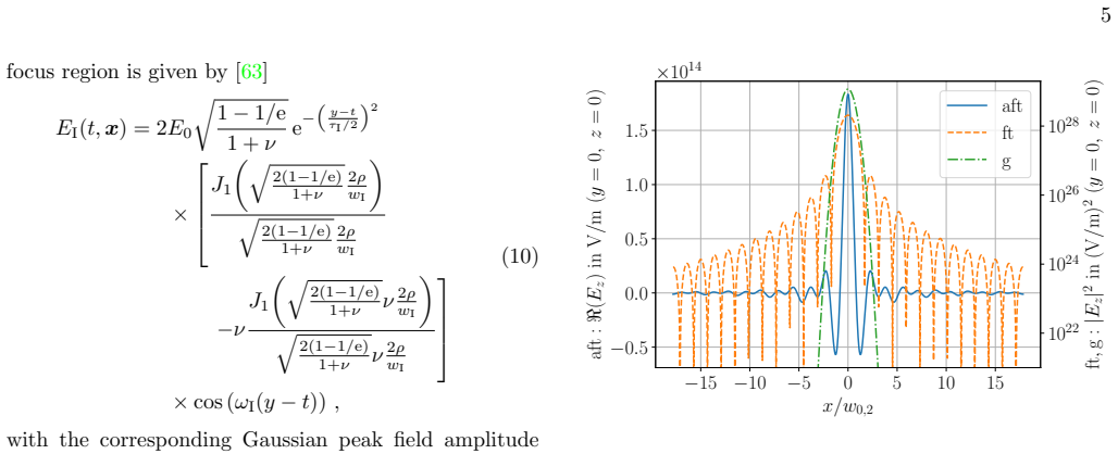
- domain assumption Annular flat-top probe field formula Eq. (10) valid in the interaction region, propagated by the Maxwell solver.
- domain assumption Infinite-Rayleigh-range approximation for analytical estimates Eqs. (13)-(15).
- ad hoc to paper Richardson extrapolation with effective convergence rate p >= 1 for all eight grid parameters, Eq. (C4).
Cite this review
Pith. "Pith review of Phase transition analogs in laser collisions with a dark-field setup." pith.science (2026). https://pith.science/paper/23ZG4F7O
@misc{pith2026241112495,
  author       = {Pith},
  title        = {Pith review of: Phase transition analogs in laser collisions with a dark-field setup},
  year         = {2026},
  howpublished = {\url{https://pith.science/paper/23ZG4F7O}},
  note         = {Machine review of arXiv:2411.12495}
}
read the original abstract
Laser pulse collisions are a promising tool for the investigation of light-by-light scattering phenomena induced by quantum vacuum fluctuations. Using the numerical code based on the vacuum emission picture and put forward in Blinne et al. (2019), we observe a strong dependence of the signal features on the transverse profiles of the colliding laser pulses in the interaction region. For a probe beam tailored such as to feature an annular far-field profile and a pronounced on-axis focus peak counterpropagating a pump beam at zero impact parameter, the signal's main emission direction can undergo the analog of a phase transition with the beam-waist ratio of the pulses serving as a control parameter. Depending on the pump's beam profile, this phase transition can be first order (e.g., for a pump with a flat-top far-field profile) or second order (e.g., for a Gaussian pump). From the simulation data, we determine the critical point and extract the corresponding critical exponent for the second-order transition of the main emission direction of the signal in the far field. For this, we improve the performance of the above numerical code, using the phase transition analogs as an example to illustrate the capabilities and limitations of the code and current workflows.
Figures


Figures from the paper (9 more)


Forward citations
Cited by 1 Pith paper
-
Back-reflection in dipole fields and beyond
Back-reflection in dipole fields is dominated by a four-wave-mixing channel; an optimized three-pulse planar setup gives ~1.5 discernible signal photons per shot with signal-to-background ~10^5.
Reference graph
Works this paper leans on
- [21]
-
[63]
F. Karbstein, Quantum Vacuum Nonlinearities in Strong Electromagnetic Fields , Habilitation thesis, Friedrich- Schiller-Universit¨at Jena (2023)
work page 2023
-
[1]
Blinne, H
A. Blinne, H. Gies, F. Karbstein, C. Kohlf ¨urst, and M. Zepf, Phys. Rev. D 99, 016006 (2019)
2019
-
[2]
Heisenberg and H
W. Heisenberg and H. Euler, Z. Phys. 98, 714 (1936)
1936
-
[3]
Weisskopf, Kong
V. Weisskopf, Kong. Dans. Vid. Selsk. Mat. Fys. Medd 14, 24 (1936)
1936
-
[4]
Dittrich and H
W. Dittrich and H. Gies, Probing the Quantum Vacuum: Perturbative Effective Action Approach in Quantum Elec- trodynamics and Its Application, Springer Tracts in Mod- ern Physics, Vol. 166 (Springer, Berlin, 2000)
2000
-
[5]
G. V. Dunne, in From Fields to Strings: Circumnavigat- ing Theoretical Physics: Ian Kogan Memorial Collection (In 3 Volumes) (World Scientific, Singapore, 2005) pp. 445–522
2005
-
[6]
Di Piazza, K
A. Di Piazza, K. Z. Hatsagortsyan, and C. H. Keitel, Phys. Rev. Lett. 100, 010403 (2008)
2008
Show all 89 references
-
[7]
Battesti and C
R. Battesti and C. Rizzo, Rep. Prog. Phys. 76, 016401 (2013)
2013
- [8]
-
[9]
Karbstein, Particles 3, 39 (2020)
F. Karbstein, Particles 3, 39 (2020)
2020
-
[10]
Fedotov, A
A. Fedotov, A. Ilderton, F. Karbstein, B. King, D. Seipt, H. Taya, and G. Torgrimsson, Phys. Rep. 1010, 1 (2023)
2023
-
[11]
Euler and B
H. Euler and B. Kockel, Naturwissenschaften 23, 246 (1935)
1935
-
[12]
Karplus and M
R. Karplus and M. Neuman, Phys. Rev. 80, 380 (1950)
1950
-
[13]
Karplus and M
R. Karplus and M. Neuman, Phys. Rev. 83, 776 (1951)
1951
-
[14]
De Tollis, Nuovo Cimento 35, 1182 (1965)
B. De Tollis, Nuovo Cimento 35, 1182 (1965)
1965
-
[15]
Lundstr ¨om, G
E. Lundstr ¨om, G. Brodin, J. Lundin, M. Marklund, R. Bingham, J. Collier, J. T. Mendon¸ ca, and P. Nor- reys, Phys. Rev. Lett. 96, 083602 (2006)
2006
-
[16]
B. King, A. Di Piazza, and C. H. Keitel, Nat. Photonics 4, 92 (2010)
2010
-
[17]
King and C
B. King and C. H. Keitel, New J. Phys.14, 103002 (2012)
2012
-
[18]
Karbstein, H
F. Karbstein, H. Gies, M. Reuter, and M. Zepf, Phys. Rev. D 92, 071301 (2015)
2015
-
[19]
Ataman, Phys
S. Ataman, Phys. Rev. A 97, 063811 (2018)
2018
-
[20]
Aboushelbaya et al
R. Aboushelbaya et al. , Phys. Rev. Lett. 123, 113604 (2019)
2019
-
[22]
C. K. Dumlu, Y. Nakamiya, and K. A. Tanaka, Phys. Rev. D 106, 116001 (2022)
2022
-
[23]
Karbstein, D
F. Karbstein, D. Ullmann, E. A. Mosman, and M. Zepf, Phys. Rev. Lett. 129, 061802 (2022)
2022
-
[24]
Sundqvist and F
C. Sundqvist and F. Karbstein, Phys. Rev. D 108, 056028 (2023)
2023
-
[25]
Formanek, J
M. Formanek, J. P. Palastro, D. Ramsey, S. Weber, and A. Di Piazza, Phys. Rev. D 109, 056009 (2024)
2024
-
[26]
A. J. Macleod and B. King, Phys. Rev. A 110, 032216 (2024)
2024
-
[27]
Sch ¨utze, L
F. Sch ¨utze, L. Doyle, J. Schreiber, M. Zepf, and F. Karb- stein, Phys. Rev. D 109, 096009 (2024)
2024
-
[28]
Peatross, J
J. Peatross, J. L. Chaloupka, and D. D. Meyerhofer, Opt. Lett. 19, 942 (1994)
1994
-
[29]
M. Zepf, G. D. Tsakiris, G. Pretzler, I. Watts, D. M. Chambers, P. A. Norreys, U. Andiel, A. E. Dangor, K. Eidmann, C. Gahn, A. Machacek, J. S. Wark, and K. Witte, Phys. Rev. E 58, R5253 (1998)
1998
- [30]
-
[31]
Gonoskov, T
A. Gonoskov, T. G. Blackburn, M. Marklund, and S. S. Bulanov, Rev. Mod. Phys. 94, 045001 (2022)
2022
-
[32]
H. Gies, F. Karbstein, and C. Kohlf ¨urst, Phys. Rev. D 97, 036022 (2018)
2018
-
[33]
B. King, H. Hu, and B. Shen, Phys. Rev. A 98, 023817 (2018)
2018
-
[34]
Karbstein, C
F. Karbstein, C. Sundqvist, K. S. Schulze, I. Uschmann, H. Gies, and G. G. Paulus, New J. Phys. 23, 095001 (2021)
2021
-
[35]
Grismayer, R
T. Grismayer, R. Torres, P. Carneiro, F. Cruz, R. Fon- seca, and L. O. Silva, New J. Phys. 23, 095005 (2021)
2021
-
[36]
Lindner, B
A. Lindner, B. ¨Olmez, and H. Ruhl, Software Impacts 15, 100481 (2023)
2023
-
[37]
A. M. Lindner, Simulating the nonlinear QED vacuum , Ph.D. thesis, Munich U. (2023)
2023
-
[38]
Galtsov and V
D. Galtsov and V. Skobelev, Phys. Lett. B 36, 238 (1971)
1971
-
[39]
Karbstein and R
F. Karbstein and R. Shaisultanov, Phys. Rev. D 91, 113002 (2015)
2015
-
[40]
Sainte-Marie, L
A. Sainte-Marie, L. Fedeli, N. Za ¨ım, F. Karbstein, and H. Vincenti, New J. Phys. 24, 065005 (2022)
2022
-
[41]
A. V. Berezin and A. M. Fedotov, Phys. Rev. D 110, 016009 (2024)
2024
-
[42]
Karbstein, A
F. Karbstein, A. Blinne, H. Gies, and M. Zepf, Phys. Rev. Lett. 123, 091802 (2019)
2019
-
[43]
Valialshchikov, F
M. Valialshchikov, F. Karbstein, D. Seipt, and M. Zepf, Phys. Rev. D 110, 076009 (2024)
2024
-
[44]
Maiwald, All-Optical Signatures of Quantum Vacuum Nonlinearities in Numerical Simulations of Unexplored Regimes, M.Sc
L. Maiwald, All-Optical Signatures of Quantum Vacuum Nonlinearities in Numerical Simulations of Unexplored Regimes, M.Sc. thesis, Friedrich-Schiller-Universit ¨at Jena, Jena (2023)
2023
-
[45]
L. P. Kadanoff, in From Order To Chaos: Essays: Criti- cal, Chaotic and Otherwise (World Scientific, Singapore,
-
[46]
K. G. Wilson and J. B. Kogut, Phys. Rep. 12, 75 (1974)
1974
-
[47]
Zinn-Justin, Int
J. Zinn-Justin, Int. Ser. Monogr. Phys. 113, 1 (2002)
2002
-
[48]
M. W. Choptuik, Phys. Rev. Lett. 70, 9 (1993)
1993
-
[49]
Gundlach and J
C. Gundlach and J. M. Martin-Garcia, Living Rev. Rel- ativity 10, 5 (2007)
2007
-
[50]
Gies and G
H. Gies and G. Torgrimsson, Phys. Rev. Lett.116, 090406 (2016)
2016
-
[51]
Gies and G
H. Gies and G. Torgrimsson, Phys. Rev. D 95, 016001 (2017)
2017
-
[52]
Ilderton, G
A. Ilderton, G. Torgrimsson, and J. W ˚ ardh, Phys. Rev. D 92, 065001 (2015)
2015
-
[53]
S. P. Gavrilov, D. M. Gitman, and A. A. Shishmarev, Phys. Rev. D 99, 116014 (2019)
2019
-
[54]
T. C. Adorno, Z.-W. He, S. P. Gavrilov, and D. M. Gitman, J. High Energy Phys. 12, 046 (2021)
2021
-
[55]
T. W. Baumgarte, B. Br ¨ugmann, D. Cors, C. Gundlach, D. Hilditch, A. Khirnov, T. Ledvinka, S. Renkhoff, and 16 I. S. Fern´ andez, Phys. Rev. Lett.131, 181401 (2023)
2023
-
[56]
D. Cors, S. Renkhoff, H. R. R ¨uter, D. Hilditch, and B. Br¨ugmann, Phys. Rev. D 108, 124021 (2023)
2023
-
[57]
Marouda, D
K. Marouda, D. Cors, H. R. R ¨uter, F. Atteneder, and D. Hilditch, Phys. Rev. D 109, 124042 (2024)
2024
-
[58]
Degli Esposti and G
G. Degli Esposti and G. Torgrimsson, Phys. Rev. D 110, 076017 (2024), arXiv:2312.17186 [hep-ph]
2024 arXiv
-
[59]
Schwinger, Phys
J. Schwinger, Phys. Rev. 82, 664 (1951)
1951
-
[60]
V. I. Ritus, Sov. Phys. JETP 42, 774 (1975)
1975
-
[61]
Dittrich and M
W. Dittrich and M. Reuter, Effective Lagrangians in Quantum Electrodynamics, Vol. 220 (Springer, New York, 1985)
1985
-
[62]
Gies and F
H. Gies and F. Karbstein, J. High Energy Phys. 2017, 108 (2017)
2017
-
[64]
Efnusheva, A
D. Efnusheva, A. Cholakoska, and A. Tentov, Int. J. Comput. Sci. Inf. Technol. 9, 151 (2017)
2017
-
[65]
“FFTW,” https://www.fftw.org/
-
[66]
Frigo and S
M. Frigo and S. Johnson, Proc. IEEE 93, 216 (2005)
2005
-
[67]
Karbstein and E
F. Karbstein and E. A. Mosman, Phys. Rev. D 100, 033002 (2019)
2019
-
[68]
Di Piazza, K
A. Di Piazza, K. Z. Hatsagortsyan, and C. H. Keitel, Phys. Rev. D 72, 085005 (2005)
2005
-
[69]
A. M. Fedotov and N. B. Narozhny, Phys. Lett. A 362, 1 (2007)
2007
-
[70]
H. Gies, F. Karbstein, and R. Shaisultanov, Phys. Rev. D 90, 033007 (2014)
2014
-
[71]
B¨ohl, B
P. B¨ohl, B. King, and H. Ruhl, Phys. Rev. A 92, 032115 (2015)
2015
-
[72]
H. Gies, F. Karbstein, and N. Seegert, Phys. Rev. D 93, 085034 (2016)
2016
-
[73]
P. V. Sasorov, F. Pegoraro, T. Z. h. Esirkepov, and S. V. Bulanov, New J. Phys. 23, 105003 (2021)
2021
-
[74]
Gori, Opt
F. Gori, Opt. Commun. 107, 335 (1994)
1994
-
[75]
L. F. Richardson, Phil. Trans. R. Soc. A 210, 307 (1911)
1911
-
[76]
Blinne, S
A. Blinne, S. Kuschel, S. Tietze, and M. Zepf, J. Comput. Phys. 1, 100019 (2019)
2019
-
[77]
“Python,” https://www.python.org/
-
[78]
“pyFFTW,” https://github.com/pyFFTW/pyFFTW
-
[79]
“Mpi4py,” https://github.com/mpi4py/mpi4py ()
-
[80]
Mpi4py-fft,
“Mpi4py-fft,” https://github.com/mpi4py/mpi4py-fft ()
-
[81]
Fast parallel multidimensional FFT using advanced MPI,
L. Dalcin, M. Mortensen, and D. E. Keyes, “Fast parallel multidimensional FFT using advanced MPI,” (2018)
2018
-
[82]
“PFFT,” https://github.com/mpip/pfft
-
[83]
Pippig, SIAM J
M. Pippig, SIAM J. Sci. Comput. 35, C213 (2013)
2013
-
[84]
P3DFFT++,
“P3DFFT++,” https://github.com/sdsc/p3dfft.3
-
[85]
Pekurovsky, SIAM J
D. Pekurovsky, SIAM J. Sci. Comput. 34, C192 (2012)
2012
-
[86]
FluidFFT,
“FluidFFT,” https://github.com/fluiddyn/fluidfft
-
[87]
A. V. Mohanan, C. Bonamy, and P. Augier, J. Open Res. Software 7, 10 (2019)
2019
-
[88]
“HeFFTe,” https://github.com/af-ayala/heffte
-
[89]
Ayala, S
A. Ayala, S. Tomov, A. Haidar, and J. Dongarra, in Computational Science – ICCS 2020 , edited by V. V. Krzhizhanovskaya, G. Z´ avodszky, M. H. Lees, J. J. Don- garra, P. M. A. Sloot, S. Brissos, and J. Teixeira (Springer International Publishing, Cham, 2020) pp. 262– 275
2020
Reviewed August 12, 2026 · model on record in the stance chip above.
Discussion (0). Continue with ORCID to comment.