REVIEW 3 major objections 5 minor 1 cited by
Enhanced Stability in Planetary Systems with Similar Masses
T0 review · 3 major / 5 minor · reviewed 2026-08-12 · deepseek-v4-flash
Pith's one-line read Planetary systems with equal-mass planets remain dynamically stable two to four orders of magnitude longer than unequal-mass systems at the same spacing, according to N-body simulations.
desk verdict Useful Gini-index stability sweep, but the headline anti-correlation is likely confounded by minimum planet mass; worth publishing after that is addressed. read the letter →
The pith
A machine-rendered reading of the paper's core claim, the machinery that carries it, and where it could break.
The reading
What carries the argument
The machinery is a controlled simulation grid: eight planets on circular, coplanar orbits around a solar-mass star, fixed total mass of 30 Earth masses, and constant spacing parameter $K=(a_{i+1}-a_i)/R_{\mathrm{H}}$ in units of the mutual Hill radius, with $K$ scanned from 3 to 10. Mass heterogeneity is quantified by the adjusted Gini index $G_m$ (0 for equal masses, approaching 1 for a dominant single planet). The dynamical explanation is carried by equipartition of random energy: since random energy is approximately $\tfrac{1}{2} m e^2/a$, equal sharing gives $e \propto m^{-1/2}$, so the smallest planets become the most eccentric and trigger the first close encounter.
What would settle it
Re-run the simulation suite with the instability threshold set to a fixed physical separation (for example, one Solar radius, or a fixed fraction of the mutual Hill radius of the encountering pair) instead of the innermost planet's Hill radius; if the two-to-four-order-of-magnitude gap between equal-mass and high-Gini systems disappears, the reported anti-correlation is an artifact of the mass-dependent definition.
Extended reading notes
Core claim
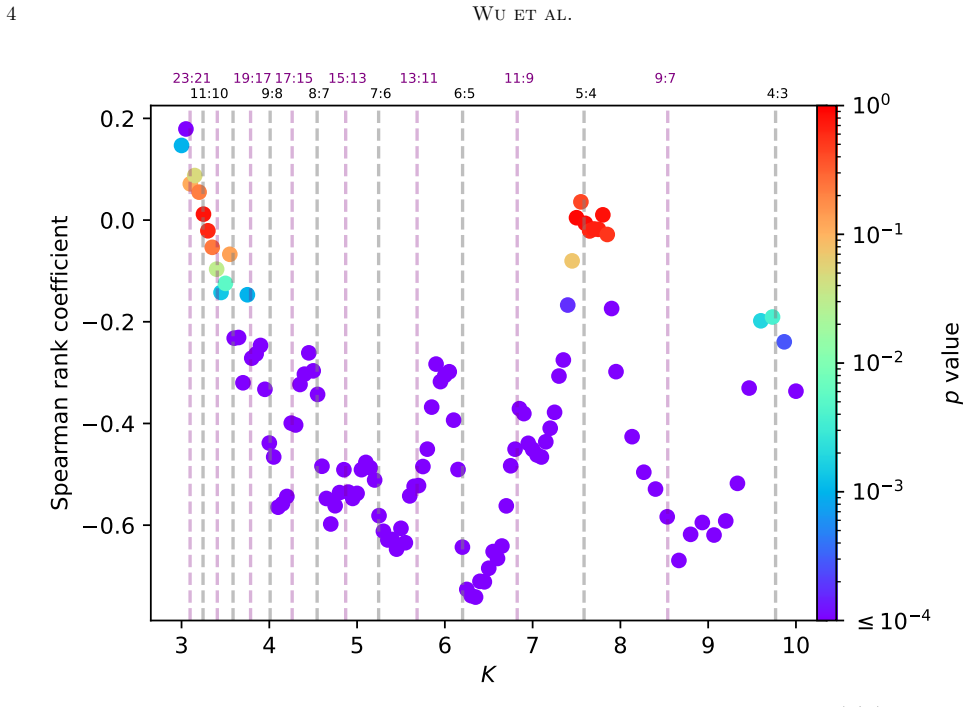
The central claim is that mass uniformity is itself a stabilising property: for non-resonant planetary systems with fixed total mass and equal spacing in units of mutual Hill radius, non-equal-mass systems are less stable than equal-mass systems. In the simulations, the scaled instability time $t/t_0$ is anti-correlated with the adjusted Gini index $G_m$ for $K>4$ away from first-order mean-motion resonances, with Spearman rank coefficients near $-0.7$ for non-resonant $K$ and $p<10^{-4}$; equal-mass systems remain stable two to four orders of magnitude longer than those with high $G_m$. Near first-order resonances the relation is non-monotonic because small mass differences shift planet pairs off exact resonance and can stabilise them. The authors attribute the destabilisation to equipartition of random energy, which gives $e \propto m^{-1/2}$, so lower-mass planets reach high eccentricities sooner. They conclude that survival bias likely contributes to the observed mass uniformity of Kepler multi-planet systems, while noting it cannot by itself explain the enhanced uniformity of near-resonant planet pairs.
Load-bearing premise
The load-bearing premise is that a close encounter closer than the Hill radius of the innermost planet marks the same 'instability' event across systems with very different mass distributions, even though that radius depends on the innermost planet's mass.
Editorial extensions
If this is right
- For observed non-resonant multi-planet systems with $K>4$, the simulations predict that the surviving population should be biased toward low $G_m$, so mass uniformity should be more common among older or more tightly packed systems.
- Near first-order mean motion resonances the trend is non-monotonic: slight mass inequality can move planet pairs off exact resonance and lengthen stability, so the anti-correlation between $t/t_0$ and $G_m$ is weaker or absent there.
- Systems with $K>8.5$ and nearly equal masses can remain stable beyond 100 Myr in these simulations, implying that such configurations are the most likely to be detected.
- The simulations stop at the first close encounter, so the reported instability times are times to first strong interaction, not to full collisional relaxation; the observed mass uniformity of near-resonant pairs ($G_m < 0.38$) is not explained by survival bias alone.
Reading between the lines
- Beyond the paper, one can test the survival-bias explanation directly by comparing the Gini index of compact multi-planet systems across stellar ages: if older systems are more mass-uniform, the bias is at work, whereas a flat age dependence would point to formation.
- Beyond the paper, the equipartition mechanism predicts that within a system about to go unstable, the smallest planet's eccentricity should grow fastest; reconstructions of eccentricity evolution in simulated or observed systems could confirm or refute this ordering.
- Beyond the paper, since the simulations terminate at first close encounter, extending them through mergers and collisions would let the final Gini index of survivors be compared with observed systems, directly quantifying how much of the 'peas-in-a-pod' pattern comes from post-instability processing.
- Beyond the paper, the dependence of the stability gap on planet number and total mass is unexplored; scaling the same constant-total-mass setup to 4, 6, or 10 planets would show whether the two-to-four-order-of-magnitude gap is generic or specific to eight-planet systems.
Editorial analysis
A structured set of objections, weighed in public.
Referee Report
Summary. This manuscript reports N-body simulations of eight-planet systems with equal mutual Hill spacing parameter K and fixed total planetary mass, varying the mass distribution as quantified by the adjusted Gini index Gm. The authors find that for K > 4 and away from first-order mean-motion resonances, the dynamical instability timescale t/t0 is anti-correlated with Gm, with high-Gm systems becoming unstable about two to four orders of magnitude sooner than equal-mass systems. They interpret this via energy equipartition (higher eccentricities in the smallest planets) and argue that survival bias may contribute to the 'peas-in-a-pod' mass uniformity observed in Kepler multi-planet systems.
Significance. If the central result is robust, it provides a simple dynamical-selection mechanism for intra-system mass uniformity that complements formation-based explanations. The paper's strengths include a well-defined integration protocol using REBOUND/Mercurius, exploration of three total masses (10, 30, and 100 Earth masses), an additional well-ordered mass configuration that addresses some observational constraints, and a clear statement of limitations in the comparison with observed near-resonant systems. The simulations are described in sufficient detail that the results are in principle reproducible, and the qualitative anti-correlation appears consistent across several K values and total masses. However, the central conclusion is currently under-supported because the analysis does not separate the effect of mass uniformity from the effect of the presence of a very low-mass planet, and because censored simulation times are treated as measured instability times in the correlation analysis.
major comments (3)
- [Section 3.2.2, Figure 2] The Spearman rank correlation in Figure 2 is computed on values of log(t/t0) where integrations that reach the maximum time of 10^8 yr are included as if they were actual instability times. For K > 8, a substantial fraction of low-Gm systems presumably survive to the maximum time, so these data points are right-censored. Treating censored values as exact times compresses the apparent distribution and can produce or exaggerate a spurious anti-correlation. The paper should either restrict the correlation analysis to K ranges with negligible censoring, use survival-analysis methods (e.g., log-rank tests or proportional hazards), or explicitly report the survival fraction as a function of Gm and K and show that the anti-correlation persists under a conservative imputation of the censored values.
- [Section 3.2.2 and Section 3.2.1] The sampling in Section 2 fixes total mass and N with only a lower bound m_i >= 0.1 Earth masses, so Gm is strongly anti-correlated with the minimum planet mass for fixed total mass and planet number. The mechanism proposed in Section 3.2.1 (Eq. 4) predicts e proportional to m^{-1/2}, so the smallest planet is expected to be the first to reach high eccentricity and trigger close encounters. Consequently, the observed anti-correlation between log(t/t0) and Gm may be fully mediated by the minimum planet mass rather than by the degree of mass uniformity. To support the general conclusion in Section 5 that 'non-equal mass systems are less stable than equal mass systems' as a statement about mass uniformity, the authors need to control for m_min, for example by generating systems with a fixed minimum mass while varying Gm, or by stratifying the correlation by m_min. Without such a test, the findings are consistent with the weaker statement that systems containing a very low-mass planet are dynamically fragile.
- [Section 2] The close encounter threshold is defined as the Hill radius of the innermost planet, Rh = a1(mu1/3)^(1/3). Because planetary masses are randomly assigned, the innermost mass varies substantially and is likely correlated with Gm: high-Gm systems often contain a very low-mass planet, and if that planet is innermost, the threshold is smaller, so a closer approach is required to register an instability. This makes the definition of t non-uniform across systems and can affect the quantitative claim of two to four orders of magnitude difference even if the qualitative anti-correlation is robust. I recommend using a pair-dependent mutual Hill radius for the encountering pair, or a fixed physical distance, and testing that the main result is insensitive to the choice of threshold.
minor comments (5)
- [Section 2] The procedure for generating mass distributions with Gm uniformly spread between 0 and 0.97 is not described; please provide the algorithm (e.g., Dirichlet-like sampling with acceptance-rejection) so that readers can reproduce the initial conditions.
- [Figure 1] The three Gm bins have different numbers of systems per K value, but the figure does not report the sample sizes in each bin or clearly define the error bars for the non-equal mass groups; please add this information in the caption or text.
- [Section 3.2.1] The equipartition argument leading to e proportional to m^{-1/2} assumes that each planet acquires a similar random energy, but the systems start on circular, coplanar orbits; the source of the initial random energy (e.g., early resonant overlap or mutual encounters) should be stated more explicitly.
- [Section 3.2.2 and Section 5] The statement that instability timescales are 'two to four orders of magnitude' longer for equal-mass systems should be accompanied by a quantitative comparison based on medians at specific K values rather than a visual estimate from Figure 1.
- [Section 4] The comparison with observed near-resonant planet pairs, which states that they generally have Gm < 0.38, would be strengthened by specifying the sample selection and the definition of 'near-resonant' used in the cited Goyal et al. (2023) work.
Circularity Check
No significant circularity: the reported Gm–stability correlation is a measured N-body output, not a derived quantity fitted to or defined by the Gini index.
full rationale
The central result is an empirical correlation between an input design variable, the adjusted Gini index Gm (Eq. 3), and an independently measured instability timescale t/t0 (Section 2: integration until a close encounter, defined by a Hill-radius threshold). No parameter is fitted to the t/t0 data and then renamed a prediction; the Spearman analysis in Section 3.2.2 summarizes simulation output rather than constructing a quantity that equals Gm by definition. The equipartition argument leading to e proportional to m^-1/2 is a post hoc explanation and is not used to define either Gm or t/t0. The only self-citations (Rice et al. 2018; Rice & Steffen 2023, co-authored by J. H. Steffen) are contextual literature references and are not load-bearing for the paper's claim. The reader and skeptic concerns about the Gm–minimum-mass coupling and the mass-dependent close-encounter threshold are confounding or validity questions, not circularity: they do not make the reported correlation equivalent to its own input by construction.
Assumptions & free parameters
free parameters (7)
- Total planetary mass =
30 Earth masses (plus 10 and 100 in extended runs)
- Number of planets =
8
- Inner semi-major axis =
0.05 AU
- Maximum integration time =
10^8 years
- Spacing parameter K range =
3 to 10
- Time step =
t0/100
- Close encounter threshold =
Hill radius of innermost planet
assumptions (5)
- domain assumption Newtonian N-body dynamics with the REBOUND Mercurius integrator accurately models the system evolution
- domain assumption Mutual Hill radius is the relevant length scale for defining spacing and stability
- domain assumption Energy equipartition applies to the planetary system, giving e proportional to m^-1/2
- domain assumption The adjusted Gini index from Goyal & Wang (2022) is a valid measure of mass uniformity
- domain assumption Initial circular, coplanar orbits are representative of post-formation planetary systems
Cite this review
Pith. "Pith review of Enhanced Stability in Planetary Systems with Similar Masses." pith.science (2026). https://pith.science/paper/5K32AHPR
@misc{pith2026241109194,
  author       = {Pith},
  title        = {Pith review of: Enhanced Stability in Planetary Systems with Similar Masses},
  year         = {2026},
  howpublished = {\url{https://pith.science/paper/5K32AHPR}},
  note         = {Machine review of arXiv:2411.09194}
}
read the original abstract
This study employs numerical simulations to explore the relationship between the dynamical instability of planetary systems and the uniformity of planetary masses within the system, quantified by the Gini index. Our findings reveal a significant correlation between system stability and mass uniformity. Specifically, planetary systems with higher mass uniformity demonstrate increased stability, particularly when they are distant from first-order mean motion resonances (MMRs). In general, for non-resonant planetary systems with a constant total mass, non-equal mass systems are less stable than equal mass systems for a given spacing in units of mutual Hill radius. This instability may arise from the equipartition of the total random energy, which can lead to higher eccentricities in smaller planets, ultimately destabilizing the system. This work suggests that the observed mass uniformity within multi-planet systems detected by \textit{Kepler} may result from a combination of survival bias and ongoing dynamical evolution processes.
Figures


Figures from the paper (2 more)


Forward citations
Cited by 1 Pith paper
-
Tidal evolution of packed moon systems around an Earth-mass planet
Including tidal migration cuts the maximum stable moon count around an Earth-mass planet to about two Moon-sized, three Pluto-sized, or five Ceres-sized moons, confined to narrow orbital-spacing windows.
Reference graph
Works this paper leans on
-
[1]
, " * write output.state after.block = add.period write newline
ENTRY address archivePrefix author booktitle chapter doi edition editor eprint howpublished institution journal key month note number organization pages publisher school series title misctitle type volume year version url label extra.label sort.label short.list INTEGERS output.state before.all mid.sentence after.sentence after.block FUNCTION init.state.co...
-
[2]
write newline
" write newline "" before.all 'output.state := FUNCTION format.doi doi empty "" "doi:" doi * if FUNCTION format.url url empty "" new.block "" url * "" * if FUNCTION format.eprint eprint empty "" archivePrefix empty "" archivePrefix ":" * if eprint field.or.null * if FUNCTION format.pid eprint empty format.doi format.eprint if FUNCTION n.dashify 't := "" t...
-
[3]
Peas in a Pod? Radius correlations in Kepler multi-planet systems
thebibliography [1] 20pt to REFERENCES 6pt =0pt -12pt 10pt plus 3pt =0pt =0pt =1pt plus 1pt =0pt =0pt -12pt =13pt plus 1pt =20pt =13pt plus 1pt \@M =10000 =-1.0em =0pt =0pt 0pt =0pt =1.0em @enumiv\@empty 10000 10000 `\.\@m \@noitemerr \@latex@warning Empty `thebibliography' environment \@ifnextchar \@reference \@latexerr Missing key on reference command E...
work page Pith review arXiv 2013
-
[4]
Adams , F. C. 2019, , 488, 1446
work page 2019
-
[5]
Adams , F. C., Batygin , K., Bloch , A. M., & Laughlin , G. 2020, , 493, 5520
work page 2020
-
[6]
2023, Nature Astronomy, 7, 330
Batygin , K., & Morbidelli , A. 2023, Nature Astronomy, 7, 330
work page 2023
-
[7]
J., Koch , D., Basri , G., et al
Borucki , W. J., Koch , D., Basri , G., et al. 2010, Science, 327, 977
2010
-
[8]
Chambers , J. E., Wetherill , G. W., & Boss , A. P. 1996, , 119, 261
work page 1996
Show all 33 references
-
[9]
M., Payne , M., & Holman , M
Deck , K. M., Payne , M., & Holman , M. J. 2013, , 774, 129
2013
-
[10]
C., Lissauer, J
Fabrycky, D. C., Lissauer, J. J., Ragozzine, D., et al. 2014, The Astrophysical Journal, 790, 146. https://dx.doi.org/10.1088/0004-637X/790/2/146
2014 doi
-
[11]
2010, , 516, A82
Funk , B., Wuchterl , G., Schwarz , R., Pilat-Lohinger , E., & Eggl , S. 2010, , 516, A82
2010
-
[12]
2024, , 527, 79
Ghosh , T., & Chatterjee , S. 2024, , 527, 79
2024
-
[13]
2022, The Astronomical Journal, 163, 201
Goldberg, M., & Batygin, K. 2022, The Astronomical Journal, 163, 201. https://dx.doi.org/10.3847/1538-3881/ac5961
2022 doi
-
[14]
V., Dai , F., & Wang , S
Goyal , A. V., Dai , F., & Wang , S. 2023, , 955, 118
2023
-
[15]
V., & Wang, S
Goyal, A. V., & Wang, S. 2022, The Astrophysical Journal, 933, 162. https://dx.doi.org/10.3847/1538-4357/ac7562
2022 doi
-
[16]
2012, Progress of Theoretical and Experimental Physics, 2012, 01A308
Kokubo, E., & Ida, S. 2012, Progress of Theoretical and Experimental Physics, 2012, 01A308. https://doi.org/10.1093/ptep/pts032
2012 doi
-
[17]
2023, , 525, L66
Lammers , C., Hadden , S., & Murray , N. 2023, , 525, L66
2023
-
[18]
J., Ragozzine, D., Fabrycky, D
Lissauer, J. J., Ragozzine, D., Fabrycky, D. C., et al. 2011, The Astrophysical Journal Supplement Series, 197, 8. https://dx.doi.org/10.1088/0067-0049/197/1/8
2011 doi
-
[19]
2014, Proceedings of the National Academy of Science, 111, 12610
Lithwick , Y., & Wu , Y. 2014, Proceedings of the National Academy of Science, 111, 12610
2014
-
[20]
2017, The Astrophysical Journal Letters, 849, L33
Millholland, S., Wang, S., & Laughlin, G. 2017, The Astrophysical Journal Letters, 849, L33. https://dx.doi.org/10.3847/2041-8213/aa9714
2017 doi
-
[21]
2021, , 656, A74
Mishra , L., Alibert , Y., Leleu , A., et al. 2021, , 656, A74
2021
-
[22]
1997, , 114, 1246
Murray , N., & Holman , M. 1997, , 114, 1246
1997
-
[23]
2017, , 293, 52
Obertas , A., Van Laerhoven , C., & Tamayo , D. 2017, , 293, 52
2017
-
[24]
F., Helled , R., & Bouchy , F
Otegi , J. F., Helled , R., & Bouchy , F. 2022, , 658, A107
2022
-
[25]
Rein , H., & Liu , S. F. 2012, , 537, A128
2012
-
[26]
M., Tamayo , D., et al
Rein , H., Hernandez , D. M., Tamayo , D., et al. 2019, , 485, 5490
2019
-
[27]
R., Rasio , F
Rice , D. R., Rasio , F. A., & Steffen , J. H. 2018, , 481, 2205
2018
-
[28]
R., & Steffen , J
Rice , D. R., & Steffen , J. H. 2023, , 520, 4057
2023
-
[29]
W., & Lissauer , J
Smith , A. W., & Lissauer , J. J. 2009, , 201, 381
2009
-
[30]
2017, Research Notes of the AAS, 1, 26
Wang, S. 2017, Research Notes of the AAS, 1, 26. https://dx.doi.org/10.3847/2515-5172/aa9be5
2017 doi
-
[31]
M., Marcy, G
Weiss, L. M., Marcy, G. W., Petigura, E. A., et al. 2018, The Astronomical Journal, 155, 48. https://dx.doi.org/10.3847/1538-3881/aa9ff6
2018 doi
-
[32]
2011, The Astrophysical Journal, 735, 109
Wu, Y., & Lithwick, Y. 2011, The Astrophysical Journal, 735, 109. https://dx.doi.org/10.1088/0004-637X/735/2/109
2011 doi
-
[33]
Zhou, J.-L., Lin, D. N. C., & Sun, Y.-S. 2007, The Astrophysical Journal, 666, 423. https://dx.doi.org/10.1086/519918
2007 doi
Reviewed August 12, 2026 · model on record in the stance chip above.
Discussion (0). Continue with ORCID to comment.