REVIEW 3 major objections 7 minor 1 cited by
Electroweak double-box integrals for Moller scattering
T0 review · 3 major / 7 minor · reviewed 2026-08-11 · deepseek-v4-flash
Pith's one-line read The paper constructs an $\varepsilon$-factorised basis for all ten planar and non-planar double-box integral families relevant to Møller scattering at NNLO, evaluating the elliptic ones as iterated integrals of elliptic periods.
desk verdict Genuinely useful two-loop integral computation; central claims hold up, weak spot is thin documentation of boundary-value and AMFlow checks. read the letter →
The pith
A machine-rendered reading of the paper's core claim, the machinery that carries it, and where it could break.
The reading
What carries the argument
The load-bearing mechanism is the $\varepsilon$-factorised (canonical) differential equation. Starting from a pre-canonical basis produced by integration-by-parts reduction, the authors seek a transformation $U$ such that $dJ=\varepsilon A J$ with $A$ independent of $\varepsilon$; the check is a direct computation of $U\tilde{A}U^{-1}-U\,dU^{-1}$. The construction is guided by maximal cuts in the Baikov representation and uses the square roots $r_1,\dots,r_8$, rationalisation variable changes, and three elliptic curves ($E(a)$ for $\tilde{B}$, $E(b)$ and $E(c)$ for $\tilde{A}$) whose periods satisfy rational differential equations in $s,t,m^2$, so the elliptic one-forms can be written without explicit root expressions. Once the basis is found, iterated integration gives the $\varepsilon$-expansion; leading large logarithms $\ln(s/m^2)$ are extracted from a single matrix and the boundary vector.
What would settle it
Evaluate any elliptic master integral, for example $J^{\tilde{A}}_{45}$ or $J^{\tilde{B}}_{61}$, at a second point well inside the region $-t \lesssim s \ll m^2$ using direct sector-wise numerical integration of the original Feynman parameter integral, and compare the $\varepsilon^0$ through $\varepsilon^4$ coefficients with the published routines. A wrong boundary constant or a region-dependent analytic continuation would show up as a mismatch at low order in $\varepsilon$, while the single benchmark point would not expose it.
Extended reading notes
Core claim
The central discovery is an explicit master-integral basis $J = U I$ for every topology, with the property $dJ = \varepsilon A J$ where $A$ depends on the kinematics but not on $\varepsilon$. The authors construct it by an educated guess informed by the maximal cut in the loop-by-loop Baikov representation and by elliptic-period calculus, then verify the factorization directly. The payoff is that the integrals can be integrated order by order in $\varepsilon$: topologies $E$ and $\tilde{E}$ reduce to harmonic polylogarithms, $B,C,D,\tilde{C},\tilde{D}$ to multiple polylogarithms after rationalising the relevant square roots, while $A$ requires iterated integrals, and the non-planar topologies $\tilde{A}$ and $\tilde{B}$ involve elliptic curves and are expressed as iterated integrals of elliptic periods. Boundary values are fixed at $t=0$, $m^2=\infty$ using power counting, vanishing conditions, and a PSLQ reconstruction over a small set of constants, after which a benchmark comparison with an independent numerical solver is reported.
Load-bearing premise
The central fragile point is the assignment of boundary constants at $t=0$, $m^2=\infty$: they are fixed partly by power counting and partially reconstructed numerically with PSLQ, and the paper validates the full set against an independent numerical solver at only one kinematic point.
Editorial extensions
If this is right
- NNLO electroweak corrections to Møller scattering can now include all double-box diagrams with three exchanged gauge bosons where at least one is a photon.
- The two elliptic non-planar topologies are no longer a separate obstruction; they are evaluated in the $\varepsilon$-expansion as iterated integrals of elliptic periods with supplied numerical routines.
- Large logarithms $\ln(s/m^2)$ at each order in $\varepsilon$ are read off from a matrix and the boundary values, giving the leading-logarithm behaviour relevant in the low-energy Møller region.
- Because the constructed basis is crossing-invariant, the same integrals cover Bhabha scattering, Drell-Yan production, and quark-pair production in $e^+e^-$ annihilation.
- The explicit basis and alphabets provide a concrete starting point for the remaining three-massive-boson double-box integrals, whose non-planar case is known to involve a genus-two curve.
Reading between the lines
- The same transformation-building pipeline could be applied to the three-massive-boson double boxes: the maximal-cut guide plus the ten-family alphabets give a concrete ansatz, but the boundary-value procedure would need an enlarged constant set beyond the seven constants used here.
- The residual boundary-value risk could be closed by deriving boundary constants from the small-$s/m^2$ expansion of the elliptic periods themselves, and by documenting the precision of the independent numerical comparison at more than one kinematic point.
- If the numerical routines are as fast as reported, the limiting step toward a complete NNLO electroweak Møller prediction becomes the remaining amplitude assembly and real-emission contributions rather than the double-box integrals.
Editorial analysis
A structured set of objections, weighed in public.
Referee Report
Summary. The paper computes the ten planar and non-planar two-loop double-box integral families that arise in NNLO electroweak corrections to Møller scattering, for configurations where three gauge bosons are exchanged between the fermion lines and at least one of them is a photon. For each topology the authors derive a differential system via IBP reduction (Kira), construct (heuristically but verifiably) an epsilon-factorised master-integral basis, fix boundary values at (t=0, m^2=infinity), and integrate the system order-by-order in epsilon. The simpler topologies are expressed in multiple polylogarithms after rationalisation of the square roots; topologies A, A-tilde and B-tilde are given as iterated integrals, with A-tilde and B-tilde involving elliptic periods. C++ numerical routines and Maple files are supplied, and the results are reported to agree perfectly with AMFlow at the benchmark point of eq. (62). Section 6 extracts the leading large logarithms ln(s/m^2), and the paper explicitly states that the existence of an epsilon-factorised basis is in general open and that its construction here is a verified guess.
Significance. The result, if correct, is a genuine step forward for NNLO electroweak corrections: it provides the first complete evaluation of the planar and non-planar double-box integrals for Møller scattering in all mass configurations with up to two massive gauge bosons, including the elliptic non-planar topologies A-tilde and B-tilde. The paper ships a complete, machine-checkable data package - transformation matrices, epsilon-factorised connection matrices, alphabets, boundary values, and C++ routines - and the epsilon-factorised property is verifiable by direct substitution into eq. (43). There are no free parameters: boundary constants are fixed by power-counting and vanishing constraints plus PSLQ over the explicit constant space of eq. (54). The reported cross-check against AMFlow, an independent implementation by a different group, anchors the calculation externally, and the authors honestly flag that a canonical basis is not guaranteed to exist and that their basis resulted from a checked heuristic. If the AMFlow comparison is quantified, I would regard the computational claims as verified rather than merely plausible.
major comments (3)
- [Section 4.2] The determination of the boundary constants at (t=0, m^2=infinity) is load-bearing, because these constants are the input to the integration of the epsilon-factorised system and a wrong boundary vector shifts every master integral at all orders. The manuscript states that PSLQ was used for 'some master integrals (of intermediate complexity)' with 'about 50 digits', but it does not specify which integrals were fixed by PSLQ, which by power counting or t-independence, what rational relations were found, and - most importantly - how the high-precision numerical values feeding PSLQ were produced (AMFlow, sector decomposition, or a series expansion at the boundary point). This provenance matters: if the boundary constants are determined from AMFlow values and the final integrals are then validated against AMFlow, the validation is partly circular; naming a different input method would break that loop. Please also address the ansatz of eq. (54): state how constants outside the Q-span of {1, i*pi, zeta2, zeta3, i*pi*zeta2, zeta4, i*pi*zeta3} (for example ln 2 from alternating MZVs in a degenerate massless or t=0 limit) were excluded, or report that PSLQ simply found no relation for such cases.
- [Section 5] The sentence 'we compared our results to the results of the program AMFlow and found perfect agreement' is not quantified. For a calculation of this size the comparison should state the number of master integrals and epsilon-orders compared, the number of agreeing digits, and the kinematic point or points used. Quantification matters for the boundary-value argument: the path-ordered exponential of an epsilon-factorised flat connection is invertible at each order in epsilon, so the epsilon^j coefficient of any master integral at a generic point equals the corresponding j-th-order boundary constant plus explicit iterated-integral terms; a high-precision check at the benchmark point of eq. (62) would therefore expose an error in any boundary constant at any order. The current one-line statement makes the strength of this check unverifiable. Please also report whether the comparison covers all master integrals or only the selection in Table 3, and consider adding a second kinematic point to guard against accidental near-degeneracies.
- [Appendix B.2.1 and B.2.2] Many master integrals of the elliptic topologies A-tilde and B-tilde are defined through functions F that are 'determined by a triangular system of first-order differential equations', with explicit expressions deferred to the supplementary files. The paper does not state the initial conditions that fix these F's at the boundary point (t=0, m^2=infinity), nor whether those initial values are part of the PSLQ/regularity fit, nor whether the modular-transformation freedom of eq. (44) was used to ensure at most simple poles at the chosen boundary point. Since the integration path starts at the boundary point, the initial values of the F's are needed for the master integrals to be uniquely defined and reproducible. Please state these initial conditions explicitly (or state unambiguously where they are imposed in the electronic files) and confirm that the boundary values of the elliptic master integrals and of the F's are mutually consistent.
minor comments (7)
- [Section 6, eqs. (66)-(67)] Eq. (66) defines the leading-log one-form as omega_tilde_1 = d ln L with L = ln(s/m^2), but eq. (67) gives J_LL = sum_j (1/j!)(epsilon L)^j M_tilde_1^j J^(0)_boundary. Solving dJ = epsilon M_tilde_1 d ln L J along the m^2-flow produces factors (epsilon ln L)^j, not (epsilon L)^j; eq. (67) is the standard solution for omega_tilde_1 = d ln(m^2) (or d ln(m^2/s)). This is likely a typo, but as printed the derivation of eq. (67) does not follow from eq. (66). Please correct the definition and ensure the electronic files define M_tilde_1 consistently with it.
- [Section 4.2] The statement 'numerical evaluations with about 50 digits are sufficient' would be more informative if the paper gave the achieved PSLQ residual and at least one representative rational relation, which would allow a reader to gauge the identification confidence.
- [Section 4.2 and Table 3] The text says boundary values follow from power counting and t-independence, which would presumably set many constants to zero; yet Table 3 shows J_A-tilde_45 and J_B-tilde_61 with vanishing terms through epsilon^3 and a non-zero epsilon^4 term. Please explain how these higher-order boundary constants are fixed, since the listed constraints alone do not obviously determine them.
- [Appendix B.2.1 and B.2.2] The definitions J_A-tilde_41, J_A-tilde_44, J_A-tilde_48 and J_B-tilde_57 involve derivatives d/dm^2 of elliptic master integrals and the Wronskians W^(X)_m2 of eq. (38); a sentence stating how these derivatives are evaluated inside the numerical routines would help readers of the C++ code.
- [Section 4.1] The elliptic one-form sets H_A-tilde and H_B-tilde appear only in the supplementary files; please state in the text at least the number of independent one-forms in each set and how they are expressed in terms of the periods and their m^2-derivatives.
- [Section 5] The claim that the evaluation routines are 'significantly faster than AMFlow' would benefit from a concrete timing example (e.g., seconds per phase-space point at a given precision).
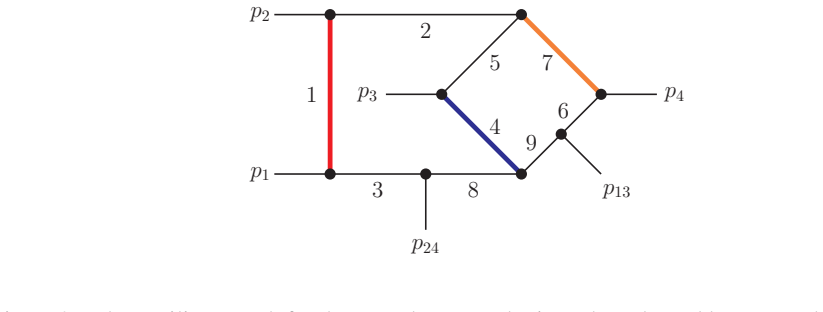
- [General presentation] Minor typographical and wording points: in Section 2.5, 'coordinates in a plane 1' should read 'coordinates in the plane' or similar; in Section 1, 'This paper is an example, how techniques...' should be 'This paper is an example of how techniques...'; and the caption of Fig. 1 could say 'photon lines' for clarity. The kinematic region is also repeated verbatim in eq. (5) and eq. (50).
Circularity Check
No circular derivation: the epsilon-factorised basis is verified by direct computation and the boundary values are checked against the independent program AMFlow; self-citations supply method and notation only.
full rationale
The derivation chain is self-contained. The claimed new result, the epsilon-factorised master-integral basis, is not defined in terms of the output: after constructing J = U I, the paper explicitly states that one computes U A~ U^-1 - U dU^-1 and checks whether epsilon factors out. This is a direct algebraic verification of eq. (15), not a fitted quantity or an imported uniqueness theorem. The boundary values at (t=0, m^2=infinity) are fixed by power counting, vanishing conditions, t-independence and PSLQ over the constant space of eq. (54); this is an internal determination of integration constants, but the final master integrals are benchmarked against AMFlow [110-112], an independent program by a different group, with the paper reporting 'perfect agreement'. The concern that the AMFlow comparison is documented only at one kinematic point and without digit counts is a correctness-risk limitation, not circularity, because AMFlow does not share the paper's fitted inputs or PSLQ ansatz. Self-citations to [81] for kinematics and notation, to [47,48,89] for elliptic-integral techniques, and to [60] for a numerical kernel supply method and implementation rather than the truth of the computed integrals; the modular-freedom remark in eqs. (44)-(45) explicitly avoids importing any uniqueness claim. No step in the paper reduces by construction to its own inputs. The score of 2 reflects only the presence of non-load-bearing self-citations, not any substantive circularity.
Assumptions & free parameters
assumptions (7)
- standard math Dimensional regularization and IBP reduction express any integral in a family as a linear combination of master integrals (refs. [82,83]).
- standard math The differential-equation method and epsilon-factorised form solve the master integrals order-by-order in epsilon (refs. [84-88]).
- standard math The elliptic curves are obtained from the maximal cut in the loop-by-loop Baikov representation (ref. [98]).
- domain assumption Electrons and neutrinos are massless, so external momenta satisfy p_i^2 = 0.
- domain assumption The physical region of interest is -t <= s << m^2 with heavy-boson mass m; the boundary point (t=0, m^2=infinity) and integration path are chosen for this region.
- domain assumption Mixed Z/W exchange between the fermion lines is excluded by the assumed initial and final states; three-massive-boson exchange is omitted due to an expected |t|/m^2 suppression.
- ad hoc to paper For each topology an epsilon-factorised basis exists and can be found by heuristic guess; the paper states this is an open question in general.
Cite this review
Pith. "Pith review of Electroweak double-box integrals for Moller scattering." pith.science (2026). https://pith.science/paper/NZ4UPVY2
@misc{pith2026241207522,
  author       = {Pith},
  title        = {Pith review of: Electroweak double-box integrals for Moller scattering},
  year         = {2026},
  howpublished = {\url{https://pith.science/paper/NZ4UPVY2}},
  note         = {Machine review of arXiv:2412.07522}
}
read the original abstract
We present for Moller scattering planar and non-planar two-loop double-box integrals where three electroweak gauge bosons are exchanged between the fermion lines, among which at least one is a photon. These integrals are relevant for the NNLO electroweak corrections to Moller scattering.
Figures


Figures from the paper (16 more)


Forward citations
Cited by 1 Pith paper
-
Analytic result of a three-loop integral family in the Higgs decay to four massive bottom quarks
Analytic master-integral results through O(ε²) are obtained for a three-loop family containing elliptic and K3 geometries by building and solving a mixed-sector ε-factorized differential equation.
Reference graph
Works this paper leans on
-
[1]
Benesch et al., (2014), arXiv:1411.4088
MOLLER, J. Benesch et al., (2014), arXiv:1411.4088
arXiv 2014
-
[2]
I. Dubovyk, A. Freitas, J. Gluza, T. Riemann, and J. Usovi tsch, Phys. Lett. B 762, 184 (2016), arXiv:1607.08375
arXiv 2016
-
[3]
Y . Du, A. Freitas, H. H. Patel, and M. J. Ramsey-Musolf, Ph ys. Rev. Lett. 126, 131801 (2021), arXiv:1912.08220
arXiv 2021
- [4]
-
[5]
I. Dubovyk et al., Phys. Rev. D 106, L111301 (2022), arXiv:2201.02576
arXiv 2022
-
[6]
T. Armadillo, R. Bonciani, S. Devoto, N. Rana, and A. Vici ni, Comput. Phys. Commun. 282, 108545 (2023), arXiv:2205.03345
arXiv 2023
-
[7]
A. G. Aleksejevs, S. G. Barkanova, Y . M. Bystritskiy, E. A . Kuraev, and V . A. Zykunov, Phys. Part. Nucl. Lett. 12, 645 (2015), arXiv:1504.03560
arXiv 2015
-
[8]
A. G. Aleksejevs, S. G. Barkanova, V . A. Zykunov, and E. A. Kuraev, Phys. Atom. Nucl. 76, 888 (2013)
2013
Show all 113 references
-
[9]
A. G. Aleksejevs et al., Eur. Phys. J. C 72, 2249 (2012)
2012
-
[10]
Delto, C
M. Delto, C. Duhr, L. Tancredi, and Y . J. Zhu, Phys. Rev. L ett. 132, 231904 (2024), arXiv:2311.06385
2024 arXiv
-
[11]
Abada et al., Eur
FCC, A. Abada et al., Eur. Phys. J. ST 228, 261 (2019)
2019
-
[12]
V . A. Smirnov, Phys. Lett. B460, 397 (1999), hep-ph/9905323
1999 arXiv
-
[13]
J. B. Tausk, Phys. Lett. B469, 225 (1999), hep-ph/9909506
1999 arXiv
-
[14]
Sabry, Nucl
A. Sabry, Nucl. Phys. 33, 401 (1962). 60
1962
-
[15]
D. J. Broadhurst, J. Fleischer, and O. Tarasov, Z.Phys. C60, 287 (1993), arXiv:hep-ph/9304303
1993 arXiv
- [16]
-
[17]
Müller-Stach, S
S. Müller-Stach, S. Weinzierl, and R. Zayadeh, Commun. Num. Theor. Phys. 6, 203 (2012), arXiv:1112.4360
2012 arXiv
-
[18]
Adams, C
L. Adams, C. Bogner, and S. Weinzierl, J. Math. Phys. 54, 052303 (2013), arXiv:1302.7004
2013 arXiv
- [19]
- [20]
-
[21]
Adams, C
L. Adams, C. Bogner, and S. Weinzierl, J. Math. Phys. 55, 102301 (2014), arXiv:1405.5640
2014 arXiv
-
[22]
Bloch, M
S. Bloch, M. Kerr, and P . V anhove, Compos. Math. 151, 2329 (2015), arXiv:1406.2664
2015 arXiv
-
[23]
Adams, C
L. Adams, C. Bogner, and S. Weinzierl, J. Math. Phys. 56, 072303 (2015), arXiv:1504.03255
2015 arXiv
-
[24]
Adams, C
L. Adams, C. Bogner, and S. Weinzierl, J. Math. Phys. 57, 032304 (2016), arXiv:1512.05630
2016 arXiv
-
[25]
Bloch, M
S. Bloch, M. Kerr, and P . V anhove, Adv. Theor. Math. Phys . 21, 1373 (2017), arXiv:1601.08181
2017 arXiv
-
[26]
Adams and S
L. Adams and S. Weinzierl, Commun. Num. Theor. Phys. 12, 193 (2018), arXiv:1704.08895
2018 arXiv
-
[27]
Bogner, A
C. Bogner, A. Schweitzer, and S. Weinzierl, Nucl. Phys. B922, 528 (2017), arXiv:1705.08952
2017 arXiv
- [28]
-
[29]
Hönemann, K
I. Hönemann, K. Tempest, and S. Weinzierl, Phys. Rev. D98, 113008 (2018), arXiv:1811.09308
2018 arXiv
- [30]
- [31]
- [32]
- [33]
-
[34]
Adams, C
L. Adams, C. Bogner, A. Schweitzer, and S. Weinzierl, J. Math. Phys. 57, 122302 (2016), arXiv:1607.01571
2016 arXiv
-
[35]
Bonciani et al., JHEP 12, 096 (2016), arXiv:1609.06685
R. Bonciani et al., JHEP 12, 096 (2016), arXiv:1609.06685
2016 arXiv
-
[36]
von Manteuffel and L
A. von Manteuffel and L. Tancredi, JHEP 06, 127 (2017), arXiv:1701.05905
2017 arXiv
-
[37]
Adams, E
L. Adams, E. Chaubey, and S. Weinzierl, Phys. Rev. Lett. 118, 141602 (2017), arXiv:1702.04279
2017 arXiv
-
[38]
Ablinger et al., J
J. Ablinger et al., J. Math. Phys. 59, 062305 (2018), arXiv:1706.01299
2018 arXiv
- [39]
-
[40]
Passarino, European Physical Journal C 77, 77 (2017), arXiv:1610.06207
G. Passarino, European Physical Journal C 77, 77 (2017), arXiv:1610.06207
2017 arXiv
- [41]
-
[42]
J. L. Bourjaily, A. J. McLeod, M. Spradlin, M. von Hippel , and M. Wilhelm, Phys. Rev. Lett. 120, 121603 (2018), arXiv:1712.02785
2018 arXiv
- [43]
-
[44]
Broedel, C
J. Broedel, C. Duhr, F. Dulat, and L. Tancredi, JHEP 05, 093 (2018), arXiv:1712.07089
2018 arXiv
-
[45]
Broedel, C
J. Broedel, C. Duhr, F. Dulat, and L. Tancredi, Phys. Rev . D97, 116009 (2018), arXiv:1712.07095
2018 arXiv
-
[46]
Broedel, C
J. Broedel, C. Duhr, F. Dulat, B. Penante, and L. Tancred i, JHEP 08, 014 (2018), arXiv:1803.10256
2018 arXiv
-
[47]
Adams, E
L. Adams, E. Chaubey, and S. Weinzierl, Phys. Rev. Lett. 121, 142001 (2018), arXiv:1804.11144
2018 arXiv
-
[48]
Adams, E
L. Adams, E. Chaubey, and S. Weinzierl, JHEP 10, 206 (2018), arXiv:1806.04981. 61
2018 arXiv
-
[49]
Broedel, C
J. Broedel, C. Duhr, F. Dulat, B. Penante, and L. Tancred i, JHEP 01, 023 (2019), arXiv:1809.10698
2019 arXiv
-
[50]
Ablinger, J
J. Ablinger, J. Blümlein, P . Marquard, N. Rana, and C. Sc hneider, Nucl. Phys. B939, 253 (2019), arXiv:1810.12261
2019 arXiv
-
[51]
Broedel, C
J. Broedel, C. Duhr, F. Dulat, B. Penante, and L. Tancred i, JHEP 05, 120 (2019), arXiv:1902.09971
2019 arXiv
- [52]
- [53]
-
[54]
Bogner, S
C. Bogner, S. Müller-Stach, and S. Weinzierl, Nucl. Phy s. B 954, 114991 (2020), arXiv:1907.01251
2020 arXiv
-
[55]
B. A. Kniehl, A. V . Kotikov, A. I. Onishchenko, and O. L. V eretin, Nucl. Phys. B948, 114780 (2019), arXiv:1907.04638
2019 arXiv
-
[56]
Broedel et al., JHEP 09, 112 (2019), arXiv:1907.03787
J. Broedel et al., JHEP 09, 112 (2019), arXiv:1907.03787
2019 arXiv
-
[57]
Abreu, M
S. Abreu, M. Becchetti, C. Duhr, and R. Marzucca, JHEP 02, 050 (2020), arXiv:1912.02747
2020 arXiv
- [58]
- [59]
-
[60]
Walden and S
M. Walden and S. Weinzierl, Comput. Phys. Commun. 265, 108020 (2021), arXiv:2010.05271
2021 arXiv
-
[61]
M. A. Bezuglov, A. I. Onishchenko, and O. L. V eretin, Nuc l. Phys. B 963, 115302 (2021), arXiv:2011.13337
2021 arXiv
-
[62]
Kristensson, M
A. Kristensson, M. Wilhelm, and C. Zhang, Phys. Rev. Let t. 127, 251603 (2021), arXiv:2106.14902
2021 arXiv
-
[63]
J. L. Bourjaily, N. Kalyanapuram, C. Langer, and K. Pata toukos, Phys. Rev. D 104, 125009 (2021), arXiv:2102.02210
2021 arXiv
-
[64]
Badger, E
S. Badger, E. Chaubey, H. B. Hartanto, and R. Marzucca, J HEP 06, 163 (2021), arXiv:2102.13450
2021 arXiv
- [65]
-
[66]
Frellesvig, JHEP 03, 079 (2022), arXiv:2110.07968
H. Frellesvig, JHEP 03, 079 (2022), arXiv:2110.07968
2022 arXiv
-
[67]
C. Duhr, V . A. Smirnov, and L. Tancredi, JHEP 09, 120 (2021), arXiv:2108.03828
2021 arXiv
- [68]
-
[69]
Morales, A
R. Morales, A. Spiering, M. Wilhelm, Q. Y ang, and C. Zhan g, Phys. Rev. Lett. 131, 041601 (2023), arXiv:2212.09762
2023 arXiv
- [70]
- [71]
-
[72]
J. L. Bourjaily et al., Functions Beyond Multiple Polylogarithms for Precision Collider Physics, in Snowmass 2021, 2022, arXiv:2203.07088
2021 arXiv
-
[73]
Jiang, X
X. Jiang, X. Wang, L. L. Y ang, and J. Zhao, JHEP 09, 187 (2023), arXiv:2305.13951
2023 arXiv
-
[74]
Frellesvig and S
H. Frellesvig and S. Weinzierl, SciPost Phys. 16, 150 (2024), arXiv:2301.02264
2024 arXiv
-
[75]
Görges, C
L. Görges, C. Nega, L. Tancredi, and F. J. Wagner, JHEP 07, 206 (2023), arXiv:2305.14090
2023 arXiv
-
[76]
Ahmed, E
T. Ahmed, E. Chaubey, M. Kaur, and S. Maggio, JHEP 05, 064 (2024), arXiv:2402.07311
2024 arXiv
-
[77]
C. Duhr, F. Gasparotto, C. Nega, L. Tancredi, and S. Wein zierl, JHEP 11, 020 (2024), arXiv:2408.05154
2024 arXiv
-
[78]
Forner, C
F. Forner, C. Nega, and L. Tancredi, (2024), arXiv:2411 .19042
2024
-
[79]
C. Duhr, F. Porkert, and S. F. Stawinski, JHEP 02, 014 (2025), arXiv:2412.02300. 62
2025
-
[80]
Marzucca, A
R. Marzucca, A. J. McLeod, B. Page, S. Pögel, and S. Weinz ierl, Phys. Rev. D 109, L031901 (2024), arXiv:2307.11497
2024 arXiv
-
[81]
Böttcher, N
N. Böttcher, N. Schwanemann, and S. Weinzierl, Eur. Phy s. J. C 84, 495 (2024), arXiv:2312.06773
2024 arXiv
-
[82]
F. V . Tkachov, Phys. Lett. B 100, 65 (1981)
1981
-
[83]
K. G. Chetyrkin and F. V . Tkachov, Nucl. Phys. B 192, 159 (1981)
1981
-
[84]
A. V . Kotikov, Phys. Lett. B 254, 158 (1991)
1991
-
[85]
A. V . Kotikov, Phys. Lett. B 267, 123 (1991), [Erratum: Phys.Lett.B 295, 409–409 (1992)]
1991
- [86]
-
[87]
Gehrmann and E
T. Gehrmann and E. Remiddi, Nucl. Phys. B 580, 485 (2000), arXiv:hep-ph/9912329
2000 arXiv
-
[88]
J. M. Henn, Phys. Rev. Lett. 110, 251601 (2013), arXiv:1304.1806
2013 arXiv
- [89]
-
[90]
Bogner and S
C. Bogner and S. Weinzierl, Int. J. Mod. Phys. A25, 2585 (2010), arXiv:1002.3458
2010 arXiv
-
[91]
Maierhöfer, J
P . Maierhöfer, J. Usovitsch, and P . Uwer, Comput. Phys. Commun. 230, 99 (2018), arXiv:1705.05610
2018 arXiv
-
[92]
Klappert, F
J. Klappert, F. Lange, P . Maierhöfer, and J. Usovitsch, Comput. Phys. Commun. 266, 108024 (2021), arXiv:2008.06494
2021 arXiv
-
[93]
A. V . Smirnov and A. V . Petukhov, Lett. Math. Phys. 97, 37 (2011), arXiv:1004.4199
2011 arXiv
-
[94]
Chen, Bull
K.-T. Chen, Bull. Amer. Math. Soc. 83, 831 (1977)
1977
-
[95]
Weinzierl, Feynman Integrals
S. Weinzierl, Feynman Integrals. A Comprehensive Treatment for Students and ResearchersUNITEXT for Physics (Springer, 2022), arXiv:2201.03593
2022 arXiv
-
[96]
O. V . Tarasov, Phys. Rev. D 54, 6479 (1996), arXiv:hep-th/9606018
1996 arXiv
-
[97]
O. V . Tarasov, Nucl. Phys. B 502, 455 (1997), arXiv:hep-ph/9703319
1997 arXiv
-
[98]
Frellesvig and C
H. Frellesvig and C. G. Papadopoulos, JHEP 04, 083 (2017), arXiv:1701.07356
2017 arXiv
-
[99]
Besier, D
M. Besier, D. V an Straten, and S. Weinzierl, Commun. Num . Theor. Phys. 13, 253 (2019), arXiv:1809.10983
2019 arXiv
-
[100]
Besier, P
M. Besier, P . Wasser, and S. Weinzierl, Comput. Phys. C ommun. 253, 107197 (2020), arXiv:1910.13251
2020 arXiv
-
[101]
H. R. P . Ferguson and R. W . Forcade, Bull. Amer. Math. So c. (N.S.) 1, 912 (1979)
1979
-
[102]
H. R. P . Ferguson and D. H. Bailey, RNR Technical Report RNR-91-032 (1992)
1992
-
[103]
Ferguson, D
H. Ferguson, D. Bailey, and S. Arno, Math. Comput. 68, 351 (1999)
1999
-
[104]
D. H. Bailey and D. J. Broadhurst, Math. Comput. 70, 1719 (2001), arXiv:math/9905048
2001
-
[105]
J. A. M. V ermaseren, Int. J. Mod. Phys. A14, 2037 (1999), hep-ph/9806280
1999 arXiv
-
[106]
Remiddi and J
E. Remiddi and J. A. M. V ermaseren, Int. J. Mod. Phys. A15, 725 (2000), hep-ph/9905237
2000 arXiv
-
[107]
A. B. Goncharov, Math. Res. Lett. 5, 497 (1998)
1998
-
[108]
J. M. Borwein, D. M. Bradley, D. J. Broadhurst, and P . Li sonek, Trans. Amer. Math. Soc. 353:3, 907 (2001), math.CA/9910045
2001
-
[109]
V ollinga and S
J. V ollinga and S. Weinzierl, Comput. Phys. Commun. 167, 177 (2005), arXiv:hep-ph/0410259
2005 arXiv
-
[110]
Liu and Y .-Q
X. Liu and Y .-Q. Ma, Comput. Phys. Commun. 283, 108565 (2023), arXiv:2201.11669
2023 arXiv
-
[111]
Liu, Y .-Q
X. Liu, Y .-Q. Ma, and C.-Y . Wang, Phys. Lett. B 779, 353 (2018), arXiv:1711.09572
2018 arXiv
-
[112]
Liu and Y .-Q
Z.-F. Liu and Y .-Q. Ma, Phys. Rev. Lett. 129, 222001 (2022), arXiv:2201.11637
2022 arXiv
-
[113]
Bauer, A
C. Bauer, A. Frink, and R. Kreckel, J. Symbolic Computa tion 33, 1 (2002), cs.sc/0004015. 63
2002
Reviewed August 11, 2026 · model on record in the stance chip above.
Discussion (0). Continue with ORCID to comment.