REVIEW 3 major objections 5 minor 41 references
Combining Machine Learning with Recurrence Analysis for resonance detection
T0 review · 3 major / 5 minor · reviewed 2026-08-10 · deepseek-v4-flash
Pith's one-line read Recurrence analysis plus a standard-map-trained LSTM can locate resonances even in a four-dimensional map where conventional visualization tools do not exist.
desk verdict Promising 2D resonance detector whose "regardless of dimensionality" claim outruns the evidence; the 4D success is one embedded-only configuration with no independent ground truth. read the letter →
The pith
A machine-rendered reading of the paper's core claim, the machinery that carries it, and where it could break.
The reading
What carries the argument
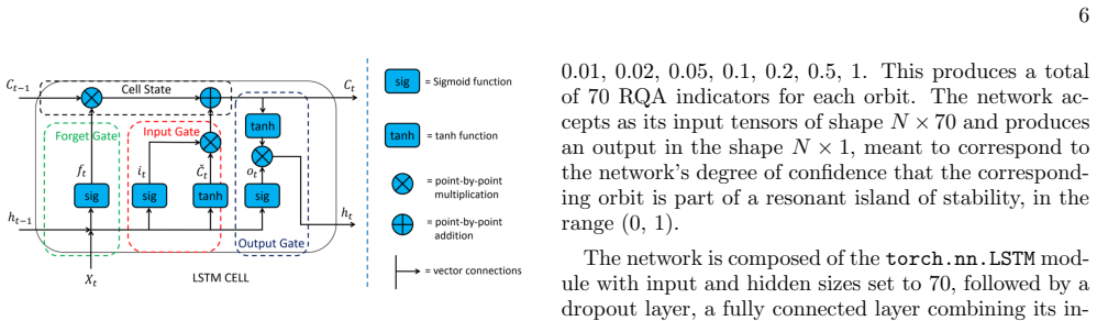
The load-bearing object is the 70-dimensional recurrence-quantification input vector: for each orbit, seven RQA measures, $RR$, $DET$, $LAM$, $L$, $L_{\rm entr}$, $DIV$, and $V_{\max}$, computed at ten recurrence thresholds $\epsilon$. These vectors, arranged as a sweep across initial conditions, are fed into a bidirectional LSTM whose cells are stacked along the initial-condition direction rather than along time. Embedding is the second mechanism: when only a scalar time series is available, time-delay embedding with dimension $m$ and delay $\tau$ reconstructs the phase space, and the paper shows that matching the embedding between training and test data is what makes the 4D detection work.
What would settle it
Compute recurrence-quantification features for the 4D map under several embedding dimensions and delays, and compare the embedded network's output peaks with the APLE resonance map: if the peak locations shift whenever $m$ or $\tau$ changes, the detections are artifacts of the embedding rather than signatures of the resonances.
Extended reading notes
Core claim
The paper's central claim is that recurrence quantifiers, the statistical measures of the diagonal and vertical line structures in a recurrence plot, carry detectable imprints of resonant islands, and that an LSTM trained once on the standard map can serve as a resonance detector for other dynamical systems, including a four-dimensional map where rotation-number and visual methods are unavailable. The basic network, trained on full phase-space coordinates, cleanly localizes resonances in two two-dimensional maps and in the Poincare section of a test particle orbiting a deformed Kerr black hole. In the 4D map, the same architecture detects resonances only when both training and test data pass through time-delay embedding: the embedded network applied to embedded data produces output peaks that align with the resonance geography charted by the APLE indicator, while the two mismatched combinations show nothing. The paper thus claims a proof of concept for a dimensionality-agnostic, automated resonance-detection pipeline, with the preprocessing convention required to match between training and application.
Load-bearing premise
The load-bearing premise is that recurrence-quantifier patterns are similar enough across different dynamical systems, when computed with the same thresholds and the same embedding choice, for a network trained on the standard map to recognize resonances in other systems; the 4D results show that this similarity holds only for matching embedding conventions.
Editorial extensions
If this is right
- Resonance localization can be automated for two-dimensional systems without manual rotation-number curves: the network trained on the standard map detects islands in the de Vogeleare map and in the black-hole Poincare section.
- For higher-dimensional systems, the practical recipe is to embed the available scalar observables and apply a network trained on embedded data; the 4D map test shows that this combination recovers the known resonance geography.
- In extreme-mass-ratio inspiral modeling, the method offers a way to identify extended resonances such as the $\omega_r/\omega_\theta = 2/3$ resonance in the Johannsen-Psaltis spacetime, helping to decide which perturbation parameters matter for waveform modeling.
- Because recurrence quantifiers are computable from any trajectory and do not require a Poincare section of a specific dimension, the same pipeline can in principle be applied to continuous-time systems by taking Poincare sections.
- The failure of the cross-combinations in the 4D experiment implies that preprocessing must be considered part of the method: a detector trained on one embedding convention is not assumed to transfer to data prepared differently.
Reading between the lines
- An implication the authors leave implicit is that the 4D success may owe more to embedding-induced features of the recurrence statistics than to a truly system-independent resonance signature; a decisive check would be to train on embedded standard-map data and test on a different embedded 4D system whose resonances are independently mapped.
- If the preprocessing-match requirement generalizes, then each new application domain will need its own embedding calibration, which weakens the 'train once, use anywhere' reading of the method.
- A testable extension for EMRI work is to apply the embedded network to synthetic gravitational-wave snapshots of inspiraling small bodies crossing a resonance and ask whether the output peaks track the crossing time; if they do, the method could become a resonance-crossing detector in waveform data.
- The hand-labeling protocol, which marks an island as resonant only if at least two neighboring initial conditions fall in it, shapes the learned target; changing the sweep spacing or labeling single-point islands could change which resonances are detected and is worth quantifying.
Editorial analysis
A structured set of objections, weighed in public.
Referee Report
Summary. The paper proposes a resonance detection method that combines recurrence quantification analysis (RQA) with a bidirectional LSTM network. The network is trained on hand-labeled orbits of the standard map and then applied to other systems: the de Vogeleare map, geodesic motion in the Johannsen-Psaltis spacetime, and a 4D symplectic map. The authors report clear resonance detection in the two 2D test cases and a partial success in the 4D case when both training and test RQA features are computed from time-delay embedded data. The stated motivation is detecting resonances in EMRI systems, where higher-dimensional phase spaces prevent the use of rotation-number methods.
Significance. Resonance detection in higher-dimensional near-integrable systems is an open problem with direct relevance to EMRI waveform modeling, and the proposed RQA+ML pipeline is a plausible and potentially useful approach. The 2D demonstrations, especially the transfer from the standard map to the de Vogeleare map and to a black-hole spacetime, are visually convincing and illustrate a practical workflow. The paper also gives a clear description of the network architecture, training data, and recurrence-analysis parameters, and it builds on standard, widely used tools. However, the central claim that recurrence quantifiers carry imprints of resonant behavior 'regardless of the system's dimensionality' rests on a single configuration in the 4D map and lacks an independent quantitative ground truth for resonance identity in that test case. As a result, the significance for EMRI applications, where more than two degrees of freedom matter, is not yet firmly established.
major comments (3)
- [Section III B and Section IV] The claim in the abstract and conclusion that recurrence quantifiers carry imprints of resonant behavior 'regardless of the system's dimensionality' is not supported by the 4D experiment as presented. The authors state in Section III B that only the embedded network applied to embedded 4D map data produces recognizable resonance peaks; the basic network on full-state 4D data fails (Fig. 9), and the cross combinations also fail. This makes the higher-dimensional success conditional on a specific embedding preprocessing pipeline, not a demonstration of a dimensionality-independent RQA signature. The conclusion 'we conclude that this method is effective' therefore overstates the strength of the 4D evidence.
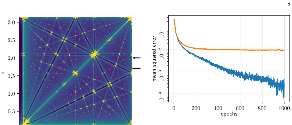
- [Section II F 3 and Section III B] There is no independent ground truth for resonance identity in the 4D map. The APLE indicator defined in Eq. (20) distinguishes regular from chaotic trajectories but does not label a regular torus as resonant or non-resonant. The statement in Section III B that 'the network is reacting to resonances in their true locations' is based on visual comparison with the APLE geography in Fig. 5, not on a quantitative resonance classification. Without an independent method to identify resonant tori in the 4D map, the peaks in Fig. 10 could be artifacts of the embedding or of the recurrence thresholds rather than universal resonance signatures.
- [Section II D and Section III B] The RQA features are computed with fixed absolute thresholds epsilon = 0.001, ..., 1 after rescaling the phase space to [0, 2*pi]^n, rather than with a fixed recurrence rate. Because the distribution of pairwise distances changes with dimensionality and after time-delay embedding, the 4D/embedded feature vectors may lie outside the feature manifold of the standard-map training data. The authors themselves show in Fig. 3 that RQA values depend strongly on the choice of epsilon. The paper should either demonstrate that the results are robust to threshold normalization, for example by using a fixed recurrence rate, or justify why absolute thresholds transfer across systems and dimensions.
minor comments (5)
- [Abstract] The sentence 'Although the tool that we are presenting here can be used is quite generic' is ungrammatical and should be revised.
- [Section II B, Eq. (5b)] In the definition of P(epsilon, v), the factors (1 - R_{i,j}) and R_{i,j+k} omit the explicit epsilon dependence that is written in Eq. (5a); the notation should be made consistent.
- [Fig. 8 caption] The caption refers to 'the 1/3 resonance is highlighted in red', while the text in Section II F 2 and Section III A 2 identifies the resonance as omega_r/omega_theta = 2/3. This inconsistency should be corrected.
- [Section II D] There is a typo in 'thetorch.nn.LSTM module'; it should read 'the torch.nn.LSTM module'.
- [Appendix A] The statement that a code release is 'under preparation' limits reproducibility; the authors should consider providing the code with the submission or at least a complete list of hyperparameters and data-generation scripts.
Circularity Check
No significant circularity: the LSTM is trained on externally hand-labeled standard-map resonances and tested on independent systems.
full rationale
The paper's derivation chain is a standard supervised-learning workflow: manual labels of resonant islands in the standard map (Sec. II E), RQA features computed from trajectories (Sec. II B), and an LSTM trained on those input-label pairs (Sec. II D). Predictions on the de Vogeleare map, the Johannsen-Psaltis Poincaré section, and the 4D map use systems and trajectories not present in training, so the test outputs are not fitted to the target data by construction. The recurrence thresholds are fixed a priori (epsilon = 0.001, ..., 1), not optimized against the test labels. The self-citations [2, 16, 17, 24, 25] provide background context, the JP metric parameters, and the 4D map definition; none is invoked as an unverified uniqueness theorem that forces the conclusion. The limitation disclosed in Sec. III B, that only the embedded-network/embedded-data combination produces recognizable peaks in the 4D map, is a generalization and validation concern (possible embedding or threshold artifacts, no quantitative ground truth for resonance identity in 4D), not a circular reduction: the network outputs are not defined in terms of the APLE curves or the recurrence quantifiers used to evaluate them. No fitted parameter is renamed as a prediction, and no derived quantity is defined in terms of the labels it is said to predict. Therefore no circularity step is present.
Assumptions & free parameters
free parameters (6)
- recurrence thresholds epsilon set =
[0.001, 0.002, 0.005, 0.01, 0.02, 0.05, 0.1, 0.2, 0.5, 1.0]
- RQA minimal line lengths lmin, vmin =
2
- embedding dimension m and delay tau for training =
m=2, tau=1
- LSTM depth and dropout rate =
depth=2, dropout=0.5
- trajectory length =
10000 points
- hand-labeling island criterion =
at least two neighboring initial conditions in island
assumptions (4)
- domain assumption Standard map dynamics capture generic resonance behavior
- standard math Takens embedding theorem guarantees faithful phase space reconstruction
- domain assumption RQA measures are sensitive to resonance identity
- ad hoc to paper LSTM can learn a mapping from RQA features to resonance membership
Cite this review
Pith. "Pith review of Combining Machine Learning with Recurrence Analysis for resonance detection." pith.science (2026). https://pith.science/paper/PYYLTO6F
@misc{pith2026241219683,
  author       = {Pith},
  title        = {Pith review of: Combining Machine Learning with Recurrence Analysis for resonance detection},
  year         = {2026},
  howpublished = {\url{https://pith.science/paper/PYYLTO6F}},
  note         = {Machine review of arXiv:2412.19683}
}
read the original abstract
The width of a resonance in a nearly integrable system, i.e. in a non-integrable system where chaotic motion is still not prominent, can tell us how a perturbation parameter is driving the system away from integrability. Although the tool that we are presenting here can be used is quite generic and can be used in a variety of systems, our particular interest lies in binary compact object systems known as extreme mass ratio inspirals (EMRIs). In an EMRI a lighter compact object, like a black hole or a neutron star, inspirals into a supermassive black hole due to gravitational radiation reaction. During this inspiral the lighter object crosses resonances, which are still not very well modeled. Measuring the width of resonances in EMRI models allows us to estimate the importance of each perturbation parameter able to drive the system away from resonances and decide whether its impact should be included in EMRI waveform modeling or not. To tackle this issue in our study we show first that recurrence quantifiers of orbits carry imprints of resonant behavior, regardless of the system's dimensionality. As a next step, we apply a long short-term memory machine learning architecture to automate the resonance detection procedure. Our analysis is developed on a simple standard map and gradually we extend it to more complicated systems until finally we employ it in a generic deformed Kerr spacetime known in the literature as the Johannsen-Psaltis spacetime.
Figures


Figures from the paper (6 more)


Reference graph
Works this paper leans on
-
[1]
With d degrees of freedom, it consists of • generalized coordinates qi, i= 1,
Hamiltonian systems Many systems in physics can be written in the form of a Hamiltonian system. With d degrees of freedom, it consists of • generalized coordinates qi, i= 1, . . . , d, • canonical momenta pi, i= 1, . . . , d, • a Hamiltonian function H qi, pi . The equations of motion then have the form dqi dt = ∂H ∂pi , (1a) dpi dt = − ∂H ∂q i . (1b) In ...
-
[2]
Dynamical maps The structure of a d = 2 Hamiltonian system’s phase space is commonly visualized using a Poincar´ e section. A surface of section is defined in the phase space such that the Hamiltonian flow is not tangent at any point of the surface, and successive intersections of the orbit and the surface of section are recorded and form the Poincar´ e s...
-
[3]
For integrals of motion we choose the values E = 0.95µ, Lz = 2 .85µM . The initial conditions are taken along the pr = 0 line on the Poincar´ e section in r ∈ [6.36M, 6.43M ] spaced at 0.001M . This sweep of initial conditions includes the ωr/ωθ = 2/3 orbital resonance
-
[4]
Dynamical mapping: de Vogeleare map For the simpler test data, we use the de Vogeleare map [23], defined as xn+1 = −yn + Kx n + x2 n , (15a) yn+1 = xn − Kx n+1 − x2 n+1 , (15b) with K ∈ R a perturbation parameter
-
[5]
Poincar´ e section: motion around a black hole One of the aims of the method developed in this pa- per is the search for extended resonances in the motion of a test particle around a black hole. Knowledge of their locations will allow us to properly model the qual- itatively distinct behavior of the passage through these resonances. We consider a particle...
-
[6]
G. Lukes-Gerakopoulos and V. Witzany, in Handbook of Gravitational Wave Astronomy , edited by C. Bambi, S. Katsanevas, and K. D. Kokkotas (2021) p. 42
work page 2021
-
[7]
Higher-dimensional example: 4D map In a Hamiltonian system with 2 degrees of freedom, alternative methods exist which can detect resonances, such as the rotation curve and its estimation using the 2-dimensional Poincar´ e section. However, already in a system with 3 degrees of freedom, the Poincar´ e section becomes 4-dimensional and these simple methods ...
-
[8]
de Vogeleare map To demonstrate the effectiveness and robustness of the resonance detection network, we apply it to test data generated by a different system than the standard map. Fig. 7 shows the results of testing on the de Vo- geleare map data. The perturbation parameter is set to K = 0 .56 and 2001 initial conditions are used with linear spacing in x...
work page 2001
Show all 41 references
-
[9]
with the machine learning approach. In the current paper, we first describe the method and demonstrate its abilities on simple systems (standard and de Voge- arXiv:2412.19683v1 [gr-qc] 27 Dec 2024 2 0 1 2 3 4 5 6 x −3 −2 −1 0 1 2 3 y Figure 1. Phase portrait of the standard ma...
2024 arXiv
-
[10]
8 shows the result of the basic network applied to the Poincar´ e section of a test particle following a geodesic in the Johannsen-Psaltis spacetime metric (see Sec
Motion around a black hole Fig. 8 shows the result of the basic network applied to the Poincar´ e section of a test particle following a geodesic in the Johannsen-Psaltis spacetime metric (see Sec. II F 2). The section contains a single resonance ωr/ωθ = 2 /3, which is detecte...
2001
-
[11]
4D map Finally, let us focus on the 4-dimensional map. Fig. 9 shows the output of the basic network over the two curves described in Sec. II F 3. For better orientation, the corresponding APLE curves are also shown. In this case, no resonances are clearly recognizable in the n...
-
[12]
S. H. Strogatz, Nonlinear Dynamics and Chaos , 2nd ed. (CRC Press, London, England, 2019)
2019
-
[13]
Mukherjee, O
S. Mukherjee, O. Kop´ aˇ cek, and G. Lukes-Gerakopoulos, Phys. Rev. D 107, 064005 (2023), arXiv:2206.10302 [gr- qc]
2023 arXiv
-
[14]
Zelenka, G
O. Zelenka, G. Lukes-Gerakopoulos, V. Witzany, and O. Kop´ aˇ cek, Phys. Rev. D101, 024037 (2020)
2020
-
[15]
Amaro-Seoane, Living Reviews in Relativity 21, 4 (2018), arXiv:1205.5240 [astro-ph.CO]
P. Amaro-Seoane, Living Reviews in Relativity 21, 4 (2018), arXiv:1205.5240 [astro-ph.CO]. 12
2018 arXiv
-
[16]
Amaro-Seoane, J
P. Amaro-Seoane, J. Andrews, M. Arca Sedda, A. Askar, Q. Baghi, R. Balasov, I. Bartos, S. S. Bav- era, J. Bellovary, C. P. L. Berry, E. Berti, S. Bianchi, L. Blecha, S. Blondin, T. Bogdanovi´ c,et al., Living Re- views in Relativity 26, 2 (2023), arXiv:2203.06016 [gr- qc]
2023 arXiv
-
[17]
Sukov´ a and O
P. Sukov´ a and O. Semer´ ak, MNRAS436, 978 (2013), arXiv:1308.4306 [gr-qc]
2013 arXiv
-
[18]
M. D. Hartl, Phys. Rev. D 67, 024005 (2003), arXiv:gr- qc/0210042 [gr-qc]
2003
-
[19]
Marwan, M
N. Marwan, M. Carmen Romano, M. Thiel, and J. Kurths, Physics Reports 438, 237 (2007)
2007
-
[20]
Johannsen and D
T. Johannsen and D. Psaltis, Phys. Rev. D 83, 124015 (2011), arXiv:1105.3191 [gr-qc]
2011 arXiv
-
[21]
A. N. Kolmogorov, Doklady Akademii Nauk SSSR 98, 527 (1954)
1954
-
[22]
V. I. Arnold, Russian Mathematical Surveys 18, 9 (1963)
1963
-
[23]
Moser, Nachrichten der Akademie der Wissenschaften in G¨ ottingen
J. Moser, Nachrichten der Akademie der Wissenschaften in G¨ ottingen. II. Mathematisch-Physikalische Klasse , 1 (1962)
1962
-
[24]
G. D. Birkhoff, Transactions of the American Mathe- matical Society 14, 14 (1913)
1913
-
[25]
Marwan, International Journal of Bifurcation and Chaos 21, 1003 (2011), arXiv:1007.2215 [nlin.CD]
N. Marwan, International Journal of Bifurcation and Chaos 21, 1003 (2011), arXiv:1007.2215 [nlin.CD]
2011 arXiv
-
[26]
Lukes-Gerakopoulos and O
G. Lukes-Gerakopoulos and O. Kop´ aˇ cek, International Journal of Modern Physics D 27, 1850010 (2018), arXiv:1709.08446 [gr-qc]
2018 arXiv
-
[27]
Kop´ aˇ cek, V
O. Kop´ aˇ cek, V. Karas, J. Kov´ aˇ r, and Z. Stuchl ´ ık, ApJ 722, 1240 (2010), arXiv:1008.4650 [astro-ph.HE]
2010 arXiv
-
[28]
Takens, in Dynamical Systems and Turbulence, War- wick 1980, edited by D
F. Takens, in Dynamical Systems and Turbulence, War- wick 1980, edited by D. Rand and L.-S. Young (Springer Berlin Heidelberg, Berlin, Heidelberg, 1981) pp. 366– 381
1980
-
[29]
Hochreiter and J
S. Hochreiter and J. Schmidhuber, Neural Computation 9, 1735 (1997), https://direct.mit.edu/neco/article- pdf/9/8/1735/813796/neco.1997.9.8.1735.pdf
1997
- [30]
-
[31]
B. V. Chirikov, Research concerning the theory of non- linear resonance and stochasticity (1971)
1971
-
[32]
Morbidelli, Modern celestial mechanics: aspects of solar system dynamics , 1st ed
A. Morbidelli, Modern celestial mechanics: aspects of solar system dynamics , 1st ed. (CRC Press, 2002)
2002
-
[33]
Reichl, The Transition to Chaos: Conservative Clas- sical Systems and Quantum Manifestations , Institute for Nonlinear Science (Springer, 2004)
L. Reichl, The Transition to Chaos: Conservative Clas- sical Systems and Quantum Manifestations , Institute for Nonlinear Science (Springer, 2004)
2004
-
[34]
Zelenka and G
O. Zelenka and G. Lukes-Gerakopoulos, in Workshop on Black Holes and Neutron Stars (2017) arXiv:1711.02442 [gr-qc]
2017 arXiv
-
[35]
Lukes-Gerakopoulos, N
G. Lukes-Gerakopoulos, N. Voglis, and C. Efthymiopou- los, Physica A: Statistical Mechanics and its Applica- tions 387, 1907 (2008)
2008
-
[36]
Froeschl´ e, M
C. Froeschl´ e, M. Guzzo, and E. Lega, Celestial Mechan- ics and Dynamical Astronomy 92, 243–255 (2005)
2005
-
[37]
D. P. Kingma and J. Ba, in 3rd International Con- ference on Learning Representations, ICLR 2015, San Diego, CA, USA, May 7-9, 2015, Conference Track Pro- ceedings, edited by Y. Bengio and Y. LeCun (2015) arXiv:1412.6980 [cs.LG]
2015 arXiv
-
[38]
Sukov´ a, M
P. Sukov´ a, M. Grzedzielski, and A. Janiuk, A& A586, A143 (2016)
2016
-
[39]
Hegger, H
R. Hegger, H. Kantz, and T. Schreiber, Chaos: An Interdisciplinary Journal of Nonlinear Science 9, 413 (1999), https://pubs.aip.org/aip/cha/article- pdf/9/2/413/18301636/413 1 online.pdf
1999
-
[40]
Marwan, Commandline recurrence plots (2006), https://tocsy.pik-potsdam.de/commandline-rp
N. Marwan, Commandline recurrence plots (2006), https://tocsy.pik-potsdam.de/commandline-rp. php
2006
-
[41]
Marwan, Recurrence plots and cross recurrence plots (2024), http://www.recurrence-plot.tk
N. Marwan, Recurrence plots and cross recurrence plots (2024), http://www.recurrence-plot.tk. Appendix A: Codes Code used to generate trajectories, train and evaluate the networks has been implemented in Python 3.11.5. The machine learning part has been done using the Py- Torc...
2024
Reviewed August 10, 2026 · model on record in the stance chip above.
Discussion (0). Continue with ORCID to comment.