REVIEW 4 major objections 4 minor 2 cited by
Black hole images under spherical-shell and circular-annulus accretion models in Schwarzschild spacetime: a semianalytical approach
T0 review · 4 major / 4 minor · reviewed 2026-08-10 · deepseek-v4-flash
Pith's one-line read The paper derives closed-form formulas for Schwarzschild black hole images under spherical-shell and circular-annulus accretion, valid at every impact parameter, and identifies a Doppler-blueshift brightening just outside the shadow for…
desk verdict Useful semianalytical extension of Gralla–Holz–Wald and Luminet, with the main risk sitting in unverified elliptic-function identities and a few fixable slips. read the letter →
The pith
A machine-rendered reading of the paper's core claim, the machinery that carries it, and where it could break.
The reading
What carries the argument
The load-bearing object is the order-by-order transfer function $r_e=h(\iota_k(\alpha,\theta_0),b)$, which assigns to a screen polar angle $\alpha$, inclination $\theta_0$, and impact parameter $b$ the radial coordinate of the $k$-th equatorial-plane crossing of the null geodesic reaching the observer; the angular map is $\iota_k(\alpha,\theta_0)=(k-1)\pi+\arccos(\tan\theta_0\cos\alpha/\sqrt{1+\tan^2\theta_0\cos^2\alpha})$. It is built from the appendix's unified lightlike-geodesic equations (A54)--(A58), which express the radial coordinate as Jacobi elliptic functions of the azimuthal angle, so that the pre- and post-periastron branches of orbits with $b>b_{\rm cri}$ no longer require separate equations and the description is valid for every impact parameter, including $b=b_{\rm cri}$. The transfer function determines the edge curves and isoradial contours of each order image, while the redshift factors $\sqrt{1-2m/r_e}$ (static), the infalling branch-dependent factors $g_f^{(\rm outw)},g_f^{(\rm inw)}$, and the rotating factor $g_r$ set the brightness, and the ratios of their fourth powers define redshift comparison functions that separate geometric from kinematic brightness differences.
What would settle it
Take a fixed inclination, say $\theta_0=\pi/3$, and for $k=1,2,3$ compute the analytic transfer function $r_e=h(\iota_k(\alpha,\theta_0),b)$ on a grid of $b$ values straddling $b_{\rm cri}$; compare each point with the radius of the $k$-th equatorial crossing obtained by direct numerical integration of $dr/d\phi = \pm (r^2/b)\sqrt{1-b^2/r^2(1-2m/r)}$. Agreement to numerical precision for $b$ just above $b_{\rm cri}$ would confirm the claimed unification, while any systematic offset would falsify it.
Extended reading notes
Core claim
On Schwarzschild spacetime, the integrated intensity on a distant observer's screen is built from three ingredients: the redshift factor $g=\nu_o/\nu_e$ for the emitter's motion, the proper length along the null geodesic inside the emitting region, and an order-by-order transfer function that maps a screen point $(b,\alpha)$ to the radial coordinate of the $k$-th intersection of the backward-traced geodesic with the equatorial plane. The paper's central claim is that all three ingredients can be given analytically for spherical-shell and circular-annulus accretion models. For the shell models, equations (2.24)--(2.29) give the observed intensity for each possible placement of the inner and outer boundaries relative to the photon orbit $r_{\rm pho}=3m$. For the annulus models, the $k$-th order transfer function $r_e=h(\iota_k(\alpha,\theta_0),b)$ works for all $b\geq 0$, matching the face-on static disk results at $\theta_0=0$ and extending the rotating-disk transfer functions, which previously held only for $b>b_{\rm cri}$. The infalling disk redshift factor is settled by locating the impact parameter $b_{\rm hal}$ at which the emitting point coincides with the periastron, so the correct branch (inward or outward segment) is used for each $b$. These formulas are the claimed generalization of the spherical- and disk-accretion images; they let a user insert any emissivity and immediately evaluate the observed integrated intensity.
Load-bearing premise
The load-bearing premise is that the appendix's rewriting of the null geodesic equations (Eqs. A54--A58) is algebraically correct for every impact parameter, from rays that never reach the photon sphere to rays that wind around the black hole many times; an error anywhere in that elliptic-function identity would invalidate the transfer functions and all intensity formulas built on them.
Editorial extensions
If this is right
- For spherical-shell accretion, equations (2.24)--(2.29) are a complete recipe: once the emissivity $j(\nu_e)$ is specified, the observed integrated intensity is a single radial integral, with the shell boundaries entering only through the integration limits and through $b_{\rm max}^{\rm SS}$ or $b_{\rm min}^{\rm SS}$.
- For circular-annulus accretion, any emission profile $I_e(r_e,\nu_e)$ can be rendered by summing the first three order images using $F_o=\sum_k g^4 \int I_e\,d\nu_e$ evaluated at $r_e=h(\iota_k,b)$, a formula that also reproduces the known face-on static images when $\theta_0=0$.
- The images imply that the shadow's dark interior is built from disjoint zero-luminosity regions in the annulus models, with its internal structure set by the inner boundary, whereas the shell-model shadow is simply the region $b<b_{\rm cri}$ with nonzero luminosity.
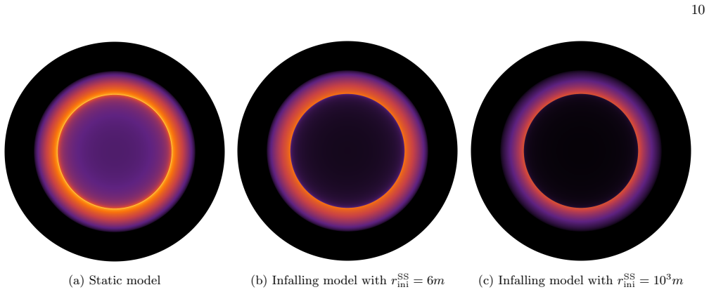
- The infalling models show Doppler redshift almost everywhere, but the region just outside the shadow is an exception for thick shells with inner boundary far from $3m$; there the luminosity is enhanced, and the enhancement grows with the initial infall radius $r_{\rm ini}^{\rm SS}$.
- The paper's correction of the $p^r$ versus $p_r$ factor in the earlier radiative-transfer formula implies that images previously built on that formula carry a systematic error, and the new spherical-shell formulas replace it.
Reading between the lines
- The paper leaves implicit that the transfer functions are purely geometric, so the same $h(\iota_k,b)$ tables would immediately render images for any alternative emissivity law--synchrotron, thermal, or line emission--without re-solving geodesics.
- A testable extension not proposed in the paper: the rim brightening (inner shell boundary far from $3m$, $b\gtrsim b_{\rm cri}$) gives a clean kinematic diagnostic, since a bright rim in a spherical-accretion image would favour fast radial inflow starting from a large initial radius.
- Carrying the same Jacobi-elliptic branch unification to Kerr spacetime is a natural next step; if it succeeds, the order-summed intensity formulas would transfer to spinning black holes with a modified redshift factor.
- Because the redshift comparison functions are independent of the emission profile, comparing two observed images of the same source at different frequencies could in principle separate gravitational lensing geometry from emitter kinematics--a separation the paper does not explicitly propose.
Signed reviews
Editorial analysis
A structured set of objections, weighed in public.
Referee Report
Summary. This paper develops semianalytical formulas for the observed integrated intensity from optically thin spherical-shell (SS) and circular-annulus (CA) accretion models in Schwarzschild spacetime. For the SS models, Eqs. (2.24)-(2.29) provide piecewise expressions for F(b) in static and infalling models for three boundary regimes, and the paper generates images for a monochromatic 1/r^2 emission profile and summarizes their geometric and luminosity features, including an infalling-model luminosity enhancement near the shadow when the inner shell boundary lies far from the photon orbit. For the CA models, Eq. (3.19) gives explicit k-th order transfer functions for all impact parameters using Jacobi elliptic functions, Eqs. (3.57)-(3.61) give integrated intensities for static, infalling, and rotating emitters, and the paper plots images for the three emission patterns of Gralla-Holz-Wald at nonzero inclination.
Significance. The paper is largely self-contained, uses a standard radiative-transfer setup, and introduces no fitted parameters: the shell and annulus radii and the infall start radii are model inputs, and the prior results used (Schwarzschild geodesics and the GHW method) are standard. If the elliptic transfer functions are correct, the CA results generalize the face-on static-disk results of Gralla, Holz, and Wald and the rotating-disk treatment of Luminet to all impact parameters and arbitrary inclination, which would be a genuinely useful technical contribution. The paper also makes concrete, boundary-dependent image predictions rather than presenting only abstract formulas, and it explicitly separates the new semianalytical framework from the specific emission patterns used for the plots. The main limitation is that the central CA formulas depend on unverified algebraic identities in the appendix, and the manuscript provides no independent numerical cross-check or code.
major comments (4)
- [Secs. II and III, Eqs. (2.16)-(2.18) and (3.49)-(3.51)] The CA transfer functions h(ι_k(α,θ0),b), the boundary curves b_min and b_max obtained from Eq. (3.20), the periastron-emission division b_hal in Eqs. (3.62)-(3.65), and the integrated intensities (3.57)-(3.61) all rest on the branch-unification identities (A52)-(A53) and the resulting geodesic equations (A54)-(A58). The manuscript gives no independent check of these identities, and the risk is concentrated in the b<b_cri and b=b_cri regimes, where the argument mixes F(ϑ_les(0), k_les) with a sign convention. I request (i) a full derivation or an explicit reference showing that (A54)-(A58) are equivalent to (A17), (A31), (A36), and (A38)-(A39) for all b, and (ii) a direct numerical ray-tracing comparison of r_e=h(ι_k(α,θ0),b) for representative values of α, b, k, and θ0, including b below and at b_cri, presented in a figure or table.
- [Sec. II.B, Eqs. (2.36)-(2.44) and Fig. 8] The momentum-component notation is internally inconsistent. Equations (2.16) and (3.49) write p^0 = -E/c = -L/b, whereas Eq. (A9) gives p^0 = E/[c(1-2m/r)]; the quantity in (2.16) is evidently the covariant component p_0. Similarly, Eq. (2.18) and its CA counterpart require p_r (not p^r) to yield the displayed sign and denominator when derived from (A9). As printed, it is not possible to verify Eqs. (2.13)-(2.15) or (3.45)-(3.47) directly from the geodesic equations without making an unstated index conversion. Please introduce p_0 and p_r consistently in these derivations and confirm that the final redshift formulas and the final integrated-intensity formulas are unchanged.
- [Sec. III.A, text after Eq. (3.19), and Sec. III.B, Eq. (3.67)] The headline enhancement near the exterior of the shadow in the infalling SS model is established by the sign of f(x_ini), but f(x_ini) is only displayed for r=7m, 15m, 23m and for ten discrete values of b above b_cri in Fig. 8. Since this is the most emphasized physical feature of the SS part of the paper, please either provide an analytic inequality proving f(x_ini)>0 in the relevant parameter range or state the parameter domain covered and test a wider grid of boundaries and impact parameters, with the numerical results made available.
- Two properties used to define the bright-region boundaries and the infalling/outgoing split are stated without proof. The monotonicity of the kth-order transfer function in b, which justifies the inequality (3.21) and the existence of unique solutions to Eq. (3.20), is inferred from Fig. 10 rather than proved. The bound b_cri ≲ b_hal(α,θ0,k) < 6m for k≥2 in Eq. (3.67) is justified by 'reading off' Fig. 2 of Ref. [44]. These properties are load-bearing for all CA image geometry, so they should be stated as lemmas with proofs, or alternatively verified numerically on a dense grid and the verification made explicit.
minor comments (4)
- [Sec. II.A, after Eq. (2.23)] The text contains several typographical errors, including 'roatating' after Eq. (3.29), 'Aa a result' and 'blushift' in Sec. III.C, and 'dependant' and 'noting' in Sec. III.C; these should be corrected.
- [Secs. II.B and IV] The statement that Ref. [34] is incorrect because p^r is replaced by p_r, and that 'relevant conclusions based on this result in a large amount of references are all faulty', is made without showing the precise replacement or its consequences. Please provide the explicit comparison or temper the claim to a specific correction.
- [Figures 12-14] Several cross-references to 'page 14' and 'page 31' are fragile and should be replaced by equation or subsection references.
- The captions state that intensities are normalized to the maximum emitted intensity I0, but they do not specify the color scaling (linear or otherwise) used in the images; please state the scaling for reproducibility.
Circularity Check
Self-contained semianalytical derivation; no fitted predictions, no load-bearing self-citations, and no step reduces by construction to its input.
full rationale
The derivation chain is self-contained. The SS and CA intensity formulas are built from the standard radiative-transfer identity (2.1)-(2.2), the redshift factors (2.13)-(2.15) and (3.45)-(3.48), which are direct evaluations of the photon-to-emitter frequency ratio from the stated emitter four-velocities, and the null-geodesic solutions (A54)-(A58) derived in the appendix from the Schwarzschild metric and standard Jacobi elliptic-function identities (A47)-(A53). No parameter is fitted: the shell/annulus boundary radii and infall-start radii are model inputs stated before the formulas, and the transfer functions (3.19) are inversions of the geodesic equation rather than fitted quantities. Prior results by Gralla-Holz-Wald and Luminet are used as benchmarks or motivations, but the load-bearing geodesic and radiative-transfer inputs are standard external results or are re-derived inside the paper. The self-citations to refs. [18,20,43] are contextual applications of ray tracing to other spacetimes and do not carry any premise of the derivation. The only substantive concern is a verification risk: the elliptic identities (A52)-(A58) are not independently machine-checked, and the infalling-model branch split at b_hal relies on their correctness. That is a correctness/robustness caveat, not circularity, since the identities are derived from the metric and elliptic-function algebra rather than assumed as the conclusion.
Assumptions & free parameters
free parameters (5)
- r_SS_inn, r_SS_out =
e.g., 2.1m to 58m
- r_SS_ini =
e.g., 2.9m to 10^3m
- r_CA_inn, r_CA_out =
e.g., 2.5m, 3m, 6m, 10m
- r_CA_ini =
e.g., 10m or infinity
- theta_0 =
0, pi/3, 4pi/9
assumptions (6)
- standard math Elliptic integrals and Jacobi elliptic function identities used in the appendix are assumed.
- domain assumption Schwarzschild spacetime is the background, and photons follow null geodesics without backreaction.
- domain assumption Accretion is optically thin, so the radiative transfer reduces to I = integral g^3 j dl with no absorption or scattering.
- domain assumption Emission is monochromatic in the emitter rest frame with specified radial profiles (1/r^2 for SS and three profiles from Gralla-Holz-Wald for CA).
- domain assumption The infalling matter moves purely radially with zero angular momentum and starts from rest at r_ini.
- domain assumption The observer is at spatial infinity, so the screen is at r = infinity and the redshift factor uses u_o^mu = (c,0,0,0).
Cite this review
Pith. "Pith review of Black hole images under spherical-shell and circular-annulus accretion models in Schwarzschild spacetime: a semianalytical approach." pith.science (2026). https://pith.science/paper/I4XZD3UR
@misc{pith2026250100361,
  author       = {Pith},
  title        = {Pith review of: Black hole images under spherical-shell and circular-annulus accretion models in Schwarzschild spacetime: a semianalytical approach},
  year         = {2026},
  howpublished = {\url{https://pith.science/paper/I4XZD3UR}},
  note         = {Machine review of arXiv:2501.00361}
}
abstract
In the static and infalling spherical-shell models of optically thin accretion on Schwarzschild black hole, the formulas for the integrated intensities observed by a distant observer are derived, and by taking the monochromatic emission pattern with a $1/r^{2}$ radial profile as example, the black hole images for the spherical shell with different boundaries are plotted. For these BH images, the geometric and luminosity features are summarized, and the qualitative explanations of the luminosity variations between the static and infalling spherical-shell models are provided. A notable feature of the black hole image in the infalling spherical-shell model is that when the inner boundary of the spherical shell is far from the bound photon orbit, the observed luminosity near the exterior of the shadow is enhanced. The circular-annulus models of optically and geometrically thin accretion on Schwarzschild black hole are further explored. For a lightlike geodesic, the analytical forms of the transfer functions working for all impact parameter values are first given, and the redshift factors in the static, infalling, and rotating circular-annulus models are then deduced. With these results, in the three situations, the formulas for the integrated intensities observed by a distant observer viewing the circular annulus at an inclination angle are derived, and the corresponding black hole images for each emission pattern provided in Phys. Rev. D \textbf{100} (2019) 024018 are plotted. Finally, for the BH images of arbitrary order, the geometric and luminosity features are also summarized, and the qualitative explanations of the luminosity variations between different CA models are also given.
Figures


Figures from the paper (13 more)


Forward citations
Cited by 2 Pith papers
-
Construction of an analytic multi-component accretion environment and its application to Kerr black hole imaging
A fully analytic accretion model combining a thick disk, Gaussian ring bumps, and localized Gaussian spots is applied to Kerr ray tracing, generating images with multiple bright spots and arcs.
-
Static Dark Fluid Thin Shells in Schwarzschild-de Sitter Spacetimes: Stability and Black Hole Shadows
Stable static dark-fluid shells separating two Schwarzschild–de Sitter spacetimes exist only for m_+/m_->1 and arise at three scales, imprinting observable black-hole shadow deviations.
Reference graph
Works this paper leans on
-
[44]
H.-Y. Pu, K. Yun, Z. Younsi, and S.-J. Yoon,Odyssey: A Public GPU-Based Code for General-Relativistic Radiative Transfer in Kerr Spacetime, Astrophys. J.820, 105 (2016)
work page 2016
-
[1]
(3.71)–(3.73), the images ofRc fs(b, α, θ0,1) in Figs
Luminosity variations throughout the entire region−π/2< α < π/2 for the first order BH images between the static and infalling CA models: From Eqs. (3.71)–(3.73), the images ofRc fs(b, α, θ0,1) in Figs. 15 and 16 indicate that within the entire region−π/2< α < π/2 of the first order BH images, the luminosity in the infalling model is always lower than tha...
-
[2]
Luminosity variations near the outer edge of the bright region for BH images of arbitrary order between the static and infalling CA models (Excluding the entire region−π/2< α < π/2 for the first order BH image): 31 From the images ofRc fs(b, α, θ0,1) andRc fs(b, α, θ0,2) in Figs. 15 and 16, if the outer boundary of the CA is sufficiently far from the boun...
-
[3]
Luminosity variations near the inner edge of the bright region for BH images of arbitrary order between the static and infalling CA models (Excluding the entire region−π/2< α < π/2 for the first order BH image): The images ofRc fs(b, α, θ0,1) andRc fs(b, α, θ0,2) in Figs. 15 and 16 also show that if the inner boundary of the CA is extended to a region nea...
-
[4]
Luminosity variations for BH images of arbitrary order between the static and rotating CA models: From the images ofRc rs(b, α, θ0,1) andRc rs(b, α, θ0,2) in Figs. 15 and 16, it is displayed that for the first and second order BH images, in a region nearα=π/2, the observed luminosities in the rotating model are lower than those in the static model, and as...
-
[5]
The original lightlike geodesic equations The metric for Schwarzschild spacetime in spherical polar coordinates (ct, r, θ, φ) is gµν = − 1− 2m r 0 0 0 0 1 1− 2m r 0 0 0 0r 2 0 0 0 0r 2 sin2 θ (A1) and four Killing vector fields in this spacetime are [50] ε0 = ∂ ∂t ,(A2) ε1 =−sinφ ∂ ∂θ −cotθcosφ ∂ ∂φ ,(A3) ε2 = cosφ ∂ ∂θ −cotθsinφ ∂ ∂...
-
[6]
When 0⩽b < bcri, the unique real root ofH(X) = 0 is X1 = 1 6 − 1 3 cosh " 2 3 arcsinh r b2 cri b2 −1 !# ,(A16) and the corresponding equation of the geodesic is ±(φ−φ 0) = s 1 2Y(X 1) −F ϑles m r , kles + F ϑles m r0 , kles (A17) 37 with ϑles(X) := arccos X−X 1 −Y(X 1) X−X 1 +Y(X 1) ! ,(A18) kles := s 1 2 + 1−6X 1 8Y(X 1) ,(A19) where Y(X 1) := p X1(3X1 −...
-
[7]
2 3 arcsin r 1− b2 cri b2 !# ,(A22) X2 = 1 6 − 1 3 cos
Whenb > bcri, the three real roots ofH(X) = 0 are X1 = 1 6 − 1 3 cos " 2 3 arcsin r 1− b2 cri b2 !# ,(A22) X2 = 1 6 − 1 3 cos " 2 3 arcsin r 1− b2 cri b2 ! − 2π 3 # ,(A23) X3 = 1 6 − 1 3 cos " 2 3 arcsin r 1− b2 cri b2 ! − 4π 3 # ,(A24) and for them, the following inequalities − 1 6 < X1 <0< X 2 < 1 3 < X3 < 1 2 (A25) hold. In this case, the form of the l...
Show all 62 references
-
[8]
Whenb=b cri, the three real roots ofH(X) = 0 under the above case reduce to X1 =− 1 6 , X 2 =X 3 = 1 3 .(A37) The two equations (A31) and (A36) are degenerated into ±(φ−φ 0) = 2 arctanh r 2m r + 1 3 −arctanh r 2m r0 + 1 3 ! ,(A38) ±(φ−φ 0) = 2 −arccoth r 2m r + 1 3 + arccoth r...
-
[9]
X1 + (X2 −X 1)sn2 ±(φ−φ 0) r X3 −X 1 2 + F ϑlarI m r0 , klar !#−1 ,(A54) r=m
Rewriting the original lightlike geodesic equations in a form suitable for practical application At present, all the ingredients to generate and analyze the BH images are available, but inspection of Eqs. (A31) and (A36) reveals that whenb > bcri, two branches of the lightlike...
-
[10]
Akiyamaet al.,First M87 Event Horizon Telescope Results
K. Akiyamaet al.,First M87 Event Horizon Telescope Results. I. The Shadow of the Supermassive Black Hole, Astrophys. J. Lett.875, L1 (2019)
2019
-
[11]
Akiyamaet al.,First M87 Event Horizon Telescope Results
K. Akiyamaet al.,First M87 Event Horizon Telescope Results. II. Array and Instrumentation, Astrophys. J. Lett.875, L2 (2019). 41
2019
-
[12]
Akiyamaet al.,First M87 Event Horizon Telescope Results
K. Akiyamaet al.,First M87 Event Horizon Telescope Results. III. Data Processing and Calibration, Astrophys. J. Lett. 875, L3 (2019)
2019
-
[13]
Akiyamaet al.,First M87 Event Horizon Telescope Results
K. Akiyamaet al.,First M87 Event Horizon Telescope Results. IV. Imaging the Central Supermassive Black Hole, Astrophys. J. Lett.875, L4 (2019)
2019
-
[14]
Akiyamaet al.,First M87 Event Horizon Telescope Results
K. Akiyamaet al.,First M87 Event Horizon Telescope Results. V. Physical Origin of the Asymmetric Ring, Astrophys. J. Lett.875, L5 (2019)
2019
-
[15]
Akiyamaet al.,First M87 Event Horizon Telescope Results
K. Akiyamaet al.,First M87 Event Horizon Telescope Results. VI. The Shadow and Mass of the Central Black Hole, Astrophys. J. Lett.875, L6 (2019)
2019
-
[16]
Akiyamaet al.,First M87 Event Horizon Telescope Results
K. Akiyamaet al.,First M87 Event Horizon Telescope Results. VII. Polarization of the Ring, Astrophys. J. Lett.910, L12 (2021)
2021
-
[17]
Akiyamaet al.,First M87 Event Horizon Telescope Results
K. Akiyamaet al.,First M87 Event Horizon Telescope Results. VIII. Magnetic Field Structure near The Event Horizon, Astrophys. J. Lett.910, L13 (2021)
2021
-
[18]
Akiyamaet al.,First Sagittarius A* Event Horizon Telescope Results
K. Akiyamaet al.,First Sagittarius A* Event Horizon Telescope Results. I. The Shadow of the Supermassive Black Hole in the Center of the Milky Way, Astrophys. J. Lett.930, L12 (2022)
2022
-
[19]
Akiyamaet al.,First Sagittarius A* Event Horizon Telescope Results
K. Akiyamaet al.,First Sagittarius A* Event Horizon Telescope Results. II. EHT and Multiwavelength Observations, Data Processing, and Calibration, Astrophys. J. Lett.930, L13 (2022)
2022
-
[20]
Akiyamaet al.,First Sagittarius A* Event Horizon Telescope Results
K. Akiyamaet al.,First Sagittarius A* Event Horizon Telescope Results. III. Imaging of the Galactic Center Supermassive Black Hole, Astrophys. J. Lett.930, L14 (2022)
2022
-
[21]
Akiyamaet al.,First Sagittarius A* Event Horizon Telescope Results
K. Akiyamaet al.,First Sagittarius A* Event Horizon Telescope Results. IV. Variability, Morphology, and Black Hole Mass, Astrophys. J. Lett.930, L15 (2022)
2022
-
[22]
Akiyamaet al.,First Sagittarius A* Event Horizon Telescope Results
K. Akiyamaet al.,First Sagittarius A* Event Horizon Telescope Results. V. Testing Astrophysical Models of the Galactic Center Black Hole, Astrophys. J. Lett.930, L16 (2022)
2022
-
[23]
Akiyamaet al.,First Sagittarius A* Event Horizon Telescope Results
K. Akiyamaet al.,First Sagittarius A* Event Horizon Telescope Results. VI. Testing the Black Hole Metric, Astrophys. J. Lett.930, L17 (2022)
2022
-
[24]
Zeng, H.-Q
X.-X. Zeng, H.-Q. Zhang, and H. Zhang,Shadows and photon spheres with spherical accretions in the four-dimensional Gauss-Bonnet black hole, Eur. Phys. J. C80, 872 (2020)
2020
-
[25]
Q. Gan, P. Wang, H. Wu, and H. Yang,Photon Spheres and Spherical Accretion Image of a Hairy Black Hole, Phys. Rev. D104, 024003 (2021)
2021
-
[26]
Guo, K.-J
S. Guo, K.-J. He, G.-R. Li, and G.-P. Li,The shadow and photon sphere of the charged black hole in Rastall gravity, Class. Quant. Grav.38, 165013 (2022)
2022
-
[27]
S. Hu, C. Deng, D. Li, X. Wu, E. Liang,Observational signatures of Schwarzschild-MOG black holes in scalar-tensor-vector gravity: shadows and rings with different accretions, Eur. Phys. J. C82, 885 (2022)
2022
-
[28]
S. Wen, W. Hong, and J. Tao,Observational Appearances of Magnetically Charged Black Holes in Born-Infeld Electrodynamics, Eur. Phys. J. C83, 277 (2023)
2023
-
[29]
S. Hu, D. Li, C. Deng, X. Wu, E. Liang,Influences of tilted thin accretion disks on the observational appearance of hairy black holes in Horndeski gravity, JCAP04, 089 (2024)
2024
-
[30]
Chandrasekhar,The Mathematical Theory of Black Holes(Oxford University Press, Oxford, 1992)
S. Chandrasekhar,The Mathematical Theory of Black Holes(Oxford University Press, Oxford, 1992)
1992
-
[31]
Cadez and U
A. Cadez and U. Kostic,Optics in the Schwarzschild space-time, Phys. Rev. D72, 104024 (2005)
2005
-
[32]
Hackmann and C
E. Hackmann and C. Lammerzahl,Geodesic equation in Schwarzschild- (anti-) de Sitter space-times: Analytical solutions and applications, Phys. Rev. D78, 024035 (2008)
2008
-
[33]
G. W. Gibbons and M. Vyska,The Application of Weierstrass elliptic functions to Schwarzschild Null Geodesics, Class. Quant. Grav.29, 065016 (2012)
2012
-
[34]
Mu˜ noz,Orbits of massless particles in the Schwarzschild metric: Exact solutions, Am
G. Mu˜ noz,Orbits of massless particles in the Schwarzschild metric: Exact solutions, Am. J. Phys.82, 564 (2014)
2014
-
[35]
Saurabh and K
K. Saurabh and K. Jusufi,Imprints of dark matter on black hole shadows using spherical accretions, Eur. Phys. J. C81, 490 (2021)
2021
-
[36]
X. Qin, S. Chen, and J. Jing,Image of a regular phantom compact object and its luminosity under spherical accretions, Class. Quant. Grav.38, 115008 (2021)
2021
-
[37]
Jusufi and Saurabh,Black hole shadows in Verlinde’s emergent gravity, Mon
K. Jusufi and Saurabh,Black hole shadows in Verlinde’s emergent gravity, Mon. Not. R. Astron. Soc.503, 1310 (2021)
2021
-
[38]
A. He, J. Tao, Y. Xue, and L. Zhang,Shadow and photon sphere of black hole in clouds of strings and quintessence, Chin. Phys. C46, 065102 (2022)
2022
-
[39]
Narayan, M
R. Narayan, M. D. Johnson, and C. F. Gammie,The Shadow of a Spherically Accreting Black Hole, Astrophys. J. Lett. 885, L33 (2019)
2019
-
[40]
Jaroszynski and A
M. Jaroszynski and A. Kurpiewski,Optics near kerr black holes: spectra of advection dominated accretion flows, Astron. Astrophys.326, 419 (1997)
1997
-
[41]
F. H. Vincent, T. Paumard, E. Gourgoulhon, and G. Perrin,GYOTO: a new general relativistic ray-tracing code, Class. Quant. Grav.28, 225011 (2011)
2011
-
[42]
Younsi, K
Z. Younsi, K. Wu, and S.V. Fuerst,General relativistic radiative transfer: formulation and emission from structured tori around black holes, Astron. Astrophys.545, A13 (2012)
2012
-
[43]
C. Bambi,Can the supermassive objects at the centers of galaxies be traversable wormholes? The first test of strong gravity for mm/sub-mm very long baseline interferometry facilities, Phys. Rev. D87, 107501 (2013)
2013
-
[45]
Luminet,Image of a spherical black hole with thin accretion disk, Astron
J.-P. Luminet,Image of a spherical black hole with thin accretion disk, Astron. Astrophys.75, 228 (1979)
1979
-
[46]
Gyulchev, P
G. Gyulchev, P. Nedkova, T. Vetsov, and S. Yazadjiev,Image of the Janis-Newman-Winicour naked singularity with a thin 42 accretion disk, Phys. Rev. D100, 024055 (2019)
2019
-
[47]
Gyulchev, P
G. Gyulchev, P. Nedkova, T. Vetsov, and S. Yazadjiev,Image of the thin accretion disk around compact objects in the Einstein-Gauss-Bonnet gravity, Eur. Phys. J. C81, 885 (2021)
2021
-
[48]
S. Paul, R. Shaikh, P. Banerjee, and T. Sarkar,Observational signatures of wormholes with thin accretion disks, JCAP 03, 055 (2020)
2020
-
[49]
Rahaman, T
F. Rahaman, T. Manna, R. Shaikh, S. Aktar, and M. Mondal,Thin accretion disks around traversable wormholes, Nucl. Phys. B.972, 115548 (2021)
2021
-
[50]
C. Liu, L. Tang, and J. Jing,Image of the Schwarzschild black hole pierced by a cosmic string with a thin accretion disk, Int. J. Mod. Phys. D31, 2250041 (2022)
2022
-
[51]
Guo, Y.-X
S. Guo, Y.-X. Huang, Y.-H. Cui, Y. Han, and Q.-Q. Jiang,Unveiling the unconventional optical signatures of regular black holes within accretion disk, Eur. Phys. J. C83, 1059 (2023)
2023
-
[52]
S. Hu, C. Deng, S. Guo, X. Wu, E. Liang,Observational signatures of Schwarzschild-MOG black holes in scalar–tensor–vector gravity: images of the accretion disk, Eur. Phys. J. C83, 264 (2023)
2023
-
[53]
S. E. Gralla, D .E. Holz, R. M. Wald,Black hole shadows, photon rings, and lensing rings, Phys. Rev. D100, 024018 (2019)
2019
-
[54]
Tian and Z.-H
S.-X. Tian and Z.-H. Zhu,Testing the Schwarzschildmetric in a strong field region with the event horizon telescope, Phys. Rev. D100, 064001 (2019)
2019
-
[55]
Gyulchev, J
G. Gyulchev, J. Kunz, P. Nedkova, T. Vetsov, and S. Yazadjiev,Observational signatures of strongly naked singularities: image of the thin accretion disk, Eur. Phys. J. C80, 1 (2020)
2020
-
[56]
M¨ uller,Analytic observation of a star orbiting a Schwarzschild black hole, Gen
T. M¨ uller,Analytic observation of a star orbiting a Schwarzschild black hole, Gen. Relativ. Gravit.41, 541 (2009)
2009
-
[57]
Bambi and E
C. Bambi and E. Barausse,Constraining the quadrupole moment of stellar-mass black-hole candidates with the continuum fitting method, Astrophys. J.731, 121 (2011)
2011
-
[58]
Bambi,A code to compute the emission of thin accretion disks in non-Kerr space-times and test the nature of black hole candidates, Astrophys
C. Bambi,A code to compute the emission of thin accretion disks in non-Kerr space-times and test the nature of black hole candidates, Astrophys. J.761, 174 (2012)
2012
-
[59]
Huang,Lectures on General Relativity(Science Press, Beijing, 2023) (in Chinese)
C.-G. Huang,Lectures on General Relativity(Science Press, Beijing, 2023) (in Chinese)
2023
-
[60]
Abramowitz and I
M. Abramowitz and I. A. Stegun,Handbook of Mathematical Functions With Formulas, Graphs, and Mathematical Tables (Courier Corporation, Washington, 1972)
1972
-
[61]
I. S. Gradshteyn and I. M. Ryzhik,Table of Integrals, Series, and Products(Academic Press, San Diego, 2007)
2007
-
[62]
J. P. Boyd,Tracing multiple solution branches for nonlinear ordinary differential equations: Chebyshev and Fourier spectral methods and a degree-increasing spectral homotopy [DISH], J. Sci. Comput.69, 1115 (2016)
2016
Reviewed August 10, 2026 · model on record in the stance chip above.
Discussion (0). Continue with ORCID to comment.