REVIEW 3 major objections 5 minor 33 references
Development of SQUID Array Amplifiers for the LiteBIRD CMB Satellite
T0 review · 3 major / 5 minor · reviewed 2026-08-10 · deepseek-v4-flash
Pith's one-line read This design study claims that a single-stage SQUID array amplifier, with tuned internal damping and shunt inductive loading, can meet LiteBIRD's readout noise and power requirements with substantial margin—about 6.3 pA/√Hz versus the 8.0…
desk verdict A careful simulation design study that makes a plausible case for single-stage SQUID amplifiers for LiteBIRD, but the 'significant engineering margin' claim is unproven until the unvaried parasitic factor and missing tolerance analysis are addressed. read the letter →
The pith
A machine-rendered reading of the paper's core claim, the machinery that carries it, and where it could break.
The reading
What carries the argument
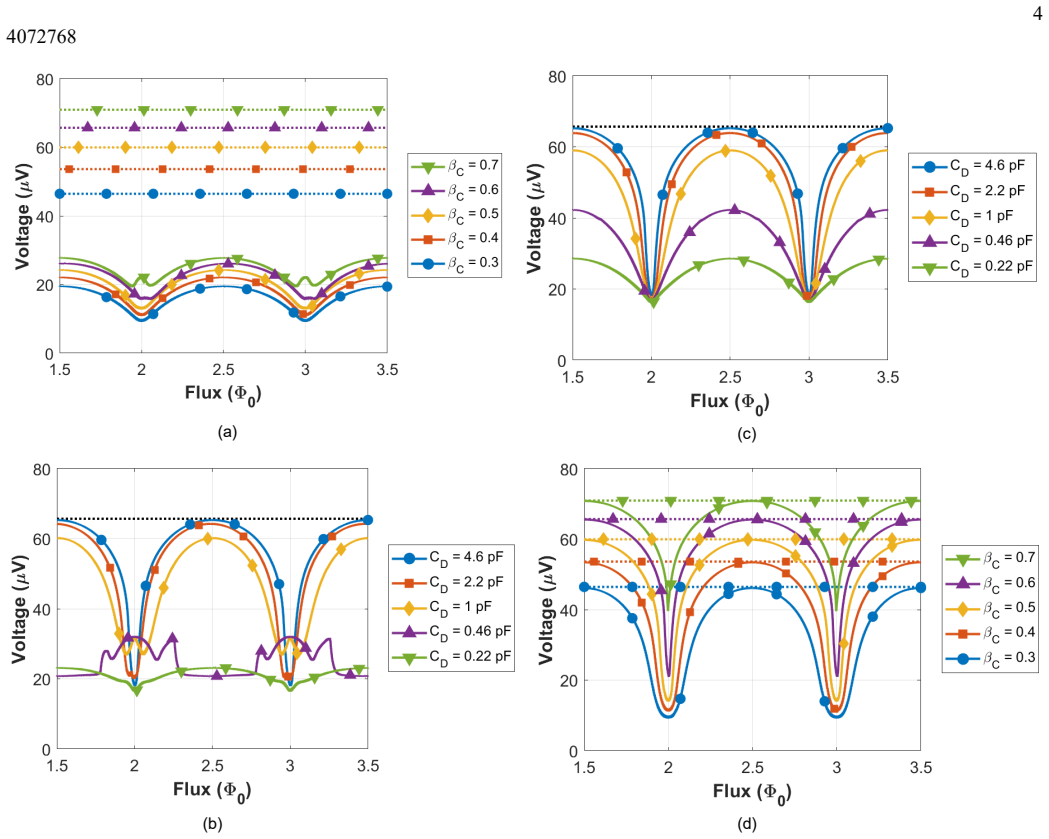
The load-bearing object is the lumped-element SQUID model implemented in LTspice, which treats each Josephson junction as a nonlinear circuit element coupled to an input transformer and to the added tuning components. The tuning mechanism is the heuristic procedure that chooses $C_{\mathrm{damping}} \approx 10~\mathrm{pF}$ and $R_{\mathrm{damping}} \approx 37~\Omega$ so the V-$\phi$ curve peaks are pulled up toward the $I_c R_{\mathrm{shunt}}$ ceiling, raising $dV/d\phi$ from about 50 to $700~\mu\mathrm{V}/\phi_0$; the added $L_{\mathrm{shunt}} = 5~\mathrm{pH}$ in series with the shunts further shapes the curves and widens the acceptable flux-bias range. The second component is the LiteBIRD readout noise model that converts the SQUID's $Z$, $L_{\mathrm{input}}$, $R_{\mathrm{dyn}}$, and input-referred current noise into the mission metric NEI_global over the 1–6 MHz multiplexing band.
What would settle it
Fabricate the tuned single-turn figure-8 SQUID array with $8~\mu\mathrm{A}/\phi_0$ input coupling, $C_{\mathrm{damping}} = 10~\mathrm{pF}$, $R_{\mathrm{damping}} = 37~\Omega$, and $L_{\mathrm{shunt}} = 5~\mathrm{pH}$, cool it to 0.4 K, and measure the input-referred current noise, transimpedance, dynamic resistance, and input inductance. Recompute the total TES-referred noise with those measured values using the same readout model; the claim stands only if the result is at or below $8.0~\mathrm{pA}/\sqrt{\mathrm{Hz}}$ while the array dissipates at most 100 nW.
Extended reading notes
Core claim
The paper's central claim is that a single-stage SQUID array amplifier can meet LiteBIRD's readout requirements if the SQUIDs are fitted with internal capacitive and resistive damping elements plus a small inductive loading on the shunt, and if the array uses a single-turn $8~\mu\mathrm{A}/\phi_0$ figure-8 input transformer. In the lumped-element simulations, these added elements restore the voltage-flux transfer function from roughly $50~\mu\mathrm{V}/\phi_0$ in the undamped baseline to roughly $700~\mu\mathrm{V}/\phi_0$, and they suppress hysteresis. When the simulated SQUID parameters are entered into the LiteBIRD readout noise model, the best tuned configurations give a total TES-referred noise-equivalent current near $6.3~\mathrm{pA}/\sqrt{\mathrm{Hz}}$ against the $8.0~\mathrm{pA}/\sqrt{\mathrm{Hz}}$ requirement while dissipating less than 100 nW. Undamped baselines all fail; among tuned configurations, only the 3-turn $24~\mu\mathrm{A}/\phi_0$ transformer fails to cross the cutoff. The paper thereby argues that the mission does not need a two-stage SQUID amplifier.
Load-bearing premise
The load-bearing assumption is that the lumped-element computer model faithfully represents the real fabricated SQUID array when cooled to 0.4 K; hidden effects such as manufacturing spread, trapped flux, or array-level resonances could consume the predicted margin.
Editorial extensions
If this is right
- LiteBIRD could baseline a single-stage SQUID array amplifier instead of a two-stage design, reducing readout complexity and cost while preserving heritage from ground-based deployments.
- The best tuned configuration provides roughly 21 percent noise margin (6.3 versus 8.0 pA/√Hz) at 4 MHz, which can absorb some fabrication variation.
- Operation at reduced power remains possible, at the cost of a narrower usable flux-bias range, giving the mission flexibility if the cryocooler budget tightens.
- Operating at lower $\beta_c$ broadens the flux-bias working area with only a slight rise in noise, which simplifies SQUID tuning.
- The 700 nm SiO2 insulator option and the 5 pH shunt inductor are retained as margin features for the initial fabrication runs.
Reading between the lines
- Going beyond the paper: a direct 0.4 K hardware test of the tuned figure-8 array is the quickest way to confirm the claimed margin, since the current evidence is entirely simulated.
- If the tuning recipe is robust, it could transfer to other sub-Kelvin frequency-multiplexed TES readout systems facing similar noise-versus-power tradeoffs.
- The single-SQUID simulations do not capture full-array resonances or crosstalk in a 58 to 68 channel multiplexer, and those effects could consume part of the predicted margin.
- The paper reports the $L_{\mathrm{shunt}}$ benefit as preliminary; a dedicated characterization of its noise penalty would make the margin estimate more secure.
Editorial analysis
A structured set of objections, weighed in public.
Referee Report
Summary. This paper reports a simulation-based design study of single-stage SQUID array amplifiers (SAAs) for the LiteBIRD CMB satellite's digital frequency multiplexing readout. The authors use LTspice lumped-element models of dc SQUIDs, with COMSOL-derived input transformer parameters and STARCryo fabrication parameters, and they develop a heuristic tuning procedure that adds capacitive damping, resistive damping, and inductive loading to the SQUID shunt circuits. For several input transformer geometries they compute the LiteBIRD noise metric NEIglobal using the public dfmux_calc tool, with the SAA characterized by transimpedance, input-referred noise, input inductance, and dynamic output resistance. They conclude that tuned single-turn 8 μA/phi0 configurations, especially a figure-8 design, can reach NEIglobal near 6.3 pA/√Hz against the 8.0 pA/√Hz requirement while dissipating under 100 nW, and that this constitutes 'significant engineering margin' for a single-stage SAA solution.
Significance. If the simulated performance is confirmed by hardware, the result would support a simpler and lower-cost single-stage SAA for LiteBIRD, avoiding the complexity of two-stage designs. The paper has clear strengths: it uses a standard circuit-simulation methodology, gives useful practical detail about LTspice convergence and timestep control, and evaluates performance with an external public tool (dfmux_calc) rather than fitting that tool's outputs in the model. The comparison across five input transformers and the explicit treatment of power dissipation versus flux-bias range are informative. The main weakness is that the central margin claim rests on an unvalidated lumped-element model and a single parasitic-inductance factor, with no fabrication-tolerance analysis and no hardware validation; the reported ~21% margin over the noise requirement is comparable to the expected size of the unmodeled effects.
major comments (3)
- [Section III] The sentence 'To roughly account for the input inductance parasitics in the SAA, Linput for the array was assumed to be N_SQUIDs × 1.1 of the SQUID Linput' is not supported by any layout analysis and is never varied. Because Linput directly controls Digital Active Nulling efficiency and therefore NEIglobal, and because the best reported value NEIglobal ≈ 6.3 pA/√Hz is only about 21% below the 8.0 pA/√Hz cutoff, a plausible increase of the parasitic factor from 1.1 to 1.3–1.5 (from inter-SQUID wiring, shunt-return paths, or kinetic inductance in the 3-μm traces) could erase the claimed margin. Please provide a sensitivity sweep over this factor and justify the 1.1 value from the physical layout.
- [Sections III, IV, VII and Fig. 4] The nominal results assume fixed STARCryo parameters (Ic = 12.6 μA, CJJ = 600 fF) and fixed tuned values (Cdamping = 10 pF, Rdamping = 37 Ω, Lshunt = 5 pH), but no fabrication-tolerance, corner, or Monte Carlo analysis is presented, and no error bars or convergence tolerances are given for the plotted NEIglobal values. Since the paper itself notes 'the propensity of SAAs toward instability and resonances' and plans to use a different SiO2 thickness for 'initial SAA fabrications', the process sensitivity is a recognized concern; yet the 'significant engineering margin' claim in the Abstract is based only on nominal simulation. A worst-case or statistical analysis over the junction, resistor, capacitor, and inductor parameters is needed to support the margin statement, or the statement should be reduced to 'meets the requirement in nominal simulation'.
- [Abstract and Section VII] The central claim of this paper is based exclusively on lumped-element LTspice simulations with no hardware validation. Unmodeled effects such as parasitic resonances, flux trapping, and fabrication spread are identified in the text as concerns, but they are not quantified. The manuscript should clearly frame the result as a design-study prediction rather than demonstrated engineering margin, and state explicitly that the 'engineering margin' refers only to margin within the simulation model. Given that the model is not yet checked against any fabricated device, this limitation is load-bearing for the main conclusion and should be prominent rather than implicit.
minor comments (5)
- [Figures 3 and 4] Axis labels, legends, and the numbers near data points are very small in the current rendering; the figures should be provided at higher resolution or with larger fonts to be readable in print.
- [Table I] The header 'turns 1/Mi' is ambiguous; please spell out the coupling quantity (e.g., 'turns' and '1/Mi (μA/phi0)') directly in the table caption and define Mi in the text.
- [Section IV] For operation at sub-Kelvin temperature, kinetic inductance in the 3-μm Nb input traces could contribute to Linput; a short quantitative estimate or a statement of why it is negligible would increase confidence in the assumed parasitic factor.
- [Notation] The paper alternates between 'NEIglobal' and 'NEI global'; please unify the notation and define the subscript or word form at first use.
- [References] The author list of reference [3] should be checked for formatting consistency; otherwise the reference list appears complete and appropriately cited.
Circularity Check
No significant circularity: the NEI_global margin is obtained from a forward-model evaluation, with damping and loading parameters chosen to maximize SQUID transfer function, not to fit the target metric.
full rationale
The paper's derivation chain is a forward simulation sequence. LTspice lumped-element SQUID simulations are used to generate V-phi curves, and the heuristic tuning procedure selects Cdamping, Rdamping, and Lshunt by maximizing V-phi amplitude and stability. The paper states: 'This procedure maximizes V-phi amplitude, stabilizes V-phi curves, and increases maximum dV/dphi at beta_c = 0.6 from ~50 uV/phi0 to ~700 uV/phi0.' The LiteBIRD performance metric NEI_global is then computed by a separate, externally provided tool: 'the Python software tool provided by LiteBIRD [14] was also run by the MATLAB controlling code, at the end of the 'flux' simulation,' using tables of Z, i_n, Linput, and Rdyn as inputs. There is no equation in the paper that defines NEI_global in terms of the tuned damping parameters by construction, and the tuning is not performed to minimize NEI_global directly. The only self-citation is dfmux_calc [14], written by co-author de Haan, but it is a public, code-reproduced forward noise model, not a fit to the paper's target result or a parameter inferred from the claimed prediction. The assumption 'Linput for the array was assumed to be NSQUIDs x 1.1 of the SQUID Linput' is an unvalidated modeling assumption, not a circular reduction; likewise the reliance on STARCryo fabrication parameters and the absence of hardware validation are correctness and risk concerns, not circularity. The central claim therefore has independent content and is not forced by definition, by fitted-input renaming, or by a self-citation chain.
Assumptions & free parameters
free parameters (4)
- Cdamping =
10 pF (for figure-8 8 µA/phi0 SQUID)
- Rdamping =
37 Ω
- Lshunt =
5 pH
- Bias operating point =
1.02 × 2Ic, beta_c = 0.6 for the main results
assumptions (7)
- domain assumption The lumped-element LTspice model with Josephson junctions as controlled sources faithfully simulates SQUID dynamics and thermal noise.
- domain assumption The Montgomery et al. circuit model for the dfMux readout represents the LiteBIRD readout system.
- domain assumption dfmux_calc, the LiteBIRD software tool, correctly computes NEI_global from SQUID parameters.
- domain assumption STARCryo fabrication parameters (Ic=12.6 µA, CJJ=600 fF, 230/300/300 nm Nb/SiO2/Nb) and COMSOL-computed transformer parameters are representative.
- domain assumption The 0 K V-phi tuning procedure yields parameters that remain near-optimal at 0.4 K with thermal noise.
- domain assumption White noise is estimated by fitting the noise power spectrum below a cutoff, typically 1 GHz.
- ad hoc to paper The SAA input inductance scales as N_SQUIDs × 1.1 × single-SQUID Linput.
Cite this review
Pith. "Pith review of Development of SQUID Array Amplifiers for the LiteBIRD CMB Satellite." pith.science (2026). https://pith.science/paper/JUZ4HYAG
@misc{pith2026250105592,
  author       = {Pith},
  title        = {Pith review of: Development of SQUID Array Amplifiers for the LiteBIRD CMB Satellite},
  year         = {2026},
  howpublished = {\url{https://pith.science/paper/JUZ4HYAG}},
  note         = {Machine review of arXiv:2501.05592}
}
read the original abstract
LiteBIRD is an upcoming JAXA-led mission that aims to measure primordial gravitational waves in the B-mode polarization of the cosmic microwave background. It is set to launch in 2032. The LiteBIRD detector array consists of around 5000 TES detectors which are read out using digital frequency multiplexing over a bandwidth of 1-6 MHz. The multiplexing factor ranges from 58x to 68x. We are presently developing single-stage SQUID array amplifiers for LiteBIRD readout. Due to the reduced complexity and cost, and greater heritage from ground-based experiments such as the South Pole Telescope and Simons Array, single-stage SQUID array amplification is preferable for the first-stage amplification, as long as it can meet the requirements. The LiteBIRD single-stage SQUID Array is required to have high transimpedance amplification while maintaining a low input inductance and low dynamic resistance. In addition, the input-referred current noise must be very low, and the power dissipation must remain below about 100 nW. These requirements have non-trivial interactions. To maximize performance within these requirements we have performed lumped-element SQUID simulation. We find that by optimizing SQUID internal damping elements and inductive loading, good single-stage SQUID array performance can be obtained for LiteBIRD, including significant engineering margin.
Figures


Figures from the paper (1 more)

Reference graph
Works this paper leans on
-
[1]
R. P. Welty and J. M. Martinis, “A series array of DC SQUIDs,” IEEE Trans. on Magn. vol. 27, no. 2, pp. 2924 -2926, 1991, https://doi.org/10.1109/20.133821
-
[2]
A. I. Braginski and J. Clarke, “Introduction,” in The SQUID handbook: Fundamentals and Technology of SQUIDs and SQUID Systems , Wiley- VCH, 2006, pp. 2-28, ISBN-13: 978-3527402298
work page 2006
-
[3]
Probing cosmic inflation with the LiteBIRD cosmic microwave background polarization survey,
LiteBIRD Collaboration, E Allys, K Arnold, J Aumont, R Aurlien, S Azzoni, et al. , “Probing cosmic inflation with the LiteBIRD cosmic microwave background polarization survey,” Prog. Theor. and Exp. Phys., Vol. 2023, Issue 4, April 2023, 042F01, https://doi.org/10.1093/ptep/ptac150
-
[4]
Thermal equilibrium calorimeters – an introduction,
D. McCammon, “Thermal equilibrium calorimeters – an introduction,” in Cryogenic Particle Detection , Springer, 2005, pp. 1 -34, ISBN -13: 978 - 3540201137
work page 2005
-
[5]
K. D. Irwin and G. C. Hilton, “Transition -Edge Sensors,” in Cryogenic Particle Detection , Springer, 2005, pp. 63 -150, ISBN -13: 978 - 3540201137
work page 2005
-
[6]
M. A. Dobbs, M. Lueker, K. A. Aird, A. N. Bender, B. A. Benson, L. E. Bleem, et al. , “Frequency multiplexed superconducting quantum interference device readout of large bolometer arrays for cosmic microwave background measurements,” Rev. Sci. Instr., vol. 83, Jul. 2012, Art. no. 073113, https://doi.org/10.1063/1.4737629
-
[7]
On -Sky Performance of the SPT -3G Frequency -Domain Multiplexed Readout,
A. N. Bender, A. J. Anderson, J. S. Avva, P. A. R. Ade, Z. Ahmed, P. S. Barry, et al. , “On -Sky Performance of the SPT -3G Frequency -Domain Multiplexed Readout,” J. Low Temp. Phys ., vol. 199, pp. 182 -191, 2020, https://doi.org/10.1007/s10909-019-02280-w
-
[8]
J. Montgomery, P. A. R. Ade, Z. Ahmed, E. Anderes, A. J. Anderson, M. Archipley, et al., “Performance and characterization of the SPT-3G digital frequency-domain multiplexed readout system using an improved noise and crosstalk model,” 2022, https://arxiv.org/abs/2103.16017v2
arXiv 2022
Show all 33 references
-
[9]
Detector and Readout Assembly and Characterization for the Simons Array,
T. Elleflot, Y. Akiba, K. Arnold, J. Avva, D. Barron, A. N. Bender, et al., “Detector and Readout Assembly and Characterization for the Simons Array,” J. Low Temp. Phys ., vol. 193, pp. 1094 -1102, 2018, https://doi.org/10.1007/s10909-018-2058-1
2018 doi
-
[10]
Two -Stage SQUID Amplifier for the Frequency Multiplexed Readout of the X -IFU X -Ray Camera,
M. Kiviranta, L. Grönberg,T. Puranen, J. van der Kuur, N. Beev, J. Salonen; D. Hazra, S. Korpela, "Two -Stage SQUID Amplifier for the Frequency Multiplexed Readout of the X -IFU X -Ray Camera," IEEE Trans. Appl. Super., vol. 31, no. 5, pp. 1 -5, Aug. 2021, Art no. 1600605, doi...
2021
-
[11]
Readout of a 176 pixel FDM system for SAFARI TES arrays
R. A. Hijmering, R. den Hartog, M. Ridder, A. J. Van Der Linden, J. Van Der Kuur, J. R. Gao, and B. Jackson. "Readout of a 176 pixel FDM system for SAFARI TES arrays." In Millimeter, Submillimeter, and Far - Infrared Detectors and Instrumentation for Astronomy VIII, vol. 9914,...
2016 doi
-
[12]
Improved performance of TES bolometers using digital feedback,
T. de Haan, G. Smecher, M. Dobbs, “Improved performance of TES bolometers using digital feedback,” Millimeter, Submillimeter, and Far - Infrared Detectors and Instrumentation for Astronomy VI , vol. 8452, pp. 113-122, 2012, https://doi.org/10.1117/12.925658
2012 doi
-
[13]
Deployment of POLARBEAR -2b,
M. Russell, K. Sakaguri, L. Ng Lowry, T. Adkins, K. Arnold, C. Baccigalupi, et al., “Deployment of POLARBEAR -2b,” J. Low Temp. Phys., vol. 216, pp. 237 -245, 2024, https://doi.org/10.1007/s10909-024- 03127-9
2024 doi
-
[14]
dfmux_calc,
T. de Haan, 2024, “dfmux_calc,” https://github.com/tijmen/dfmux_calc
2024
-
[15]
https://ngspice.sourceforge.io/docs/ngspice-html-manual/manual.xhtml
-
[16]
https://pyspice.fabrice-salvaire.fr
-
[17]
Development of frequency domain multiplexing readout using sub -kelvin SQUIDs for LiteBIRD,
M. Russell, K. Arnold, T. Elleflot, T. de Haan, J. Hubmayr, G. Jaehnig, A. Lee, J. Montgomery, and A. Suzuki. “Development of frequency domain multiplexing readout using sub -kelvin SQUIDs for LiteBIRD,” Millimeter, Submillimeter, and Far -Infrared Detectors and Instrumentatio...
2022 doi
-
[18]
A computer model for noise in the DC SQUID,
C. D. Tesche and J. Clarke, “A computer model for noise in the DC SQUID,” IEEE Trans. Mag., vol. MAG-13, no. 1, pp. 859-861, Jan. 1977, https://doi.org/10.1109/tmag.1977.1059276
1977
-
[19]
DC SQUID: noise and optimization,
C. D. Tesche and J. Clarke, “DC SQUID: noise and optimization,” J. Low Temp. Phys., vol. 29, pp. 301-331, 1977, https://doi.org/10.1007/BF00655097. 7 4072768
1977 doi
-
[20]
Analysis of a double-loop dc SQUID,
C. D. Tesche, “Analysis of a double-loop dc SQUID,” J. Low Temp. Phys., vol. 47, no. 5, pp. 385-410, 1982, https://doi.org/10.1007/bf00683981
1982 doi
-
[21]
Practical dc SQUIDs with extremely low 1/f noise,
C. Tesche, K. Brown, A. Callegari, M. Chen, J. Greiner, H. Jones, et al, “Practical dc SQUIDs with extremely low 1/f noise,” IEEE Trans. on Magn., vol. 21, no. 2, pp. 1032-1035, 1985, https://doi.org/10.1109/tmag.1985.1063725
1985
-
[22]
Ryhänen, H
T. Ryhänen, H. Seppä, and R. Cantor,”Effect of parasitic capacitance and inductance on the dynamics and noise of dc superconducting quantum interference devices,” J. Appl. Phys., vol. 71, no. 12, pp. 6150-6166, 1992, https://doi.org/10.1063/1.350424
1992 doi
-
[23]
Noise characteristics of a dc SQUID with a resistively shunted inductance,
K. Enpuku, T. Muta, K. Yoshida, and F. Irie, “Noise characteristics of a dc SQUID with a resistively shunted inductance,” J. Appl. Phys., vol. 58, no. 5, pp. 1916-1923, 1985, https://doi.org/10.1063/1.335998
1916 doi
-
[24]
Effect of damping resistance on voltage versus flux relation of a dc SQUID with large inductance and critical current,
K. Enpuku, K. Sueoka, K. Yoshida, and F. Irie, “Effect of damping resistance on voltage versus flux relation of a dc SQUID with large inductance and critical current,” J. Appl. Phys., vol. 57, no. 5, pp. 1691- 1697, 1985, https://doi.org/10.1063/1.334439
1985 doi
-
[25]
Multisim 14.3, from National Instruments, https://www.ni.com/en/support/downloads/software- products/download.multisim.html?srsltid=AfmBOopQzBh0zwCmqujLN HheuIX34Yc0Xy3Hy3vRx8CJwV8syVwPGpXv#452133
-
[26]
NGSPICE, open source, https://ngspice.sourceforge.io/
-
[27]
LTspice 17, from Analog Design, https://ez.analog.com/design-tools- and-calculators/ltspice
- [28]
-
[29]
COMSOL 6.2, https://www.comsol.com/
-
[30]
+1 505.424.6454 https://starcryo.com
STAR Cryoelectronics, 25A Bisbee Ct, Santa Fe, NM 87508 USA. +1 505.424.6454 https://starcryo.com
-
[31]
Highly sensitive and easy-to-use SQUID sensors,
D. Drung, C. Assmann, J. Beyer, A. Kirste, M. Peters, F. Ruede, and Th Schurig, “Highly sensitive and easy-to-use SQUID sensors,” IEEE Trans. Appl. Super. , vol. 17, no. 2, pp. 699 -704, 2007, https://doi.org/10.1109/tasc.2007.897403
2007
-
[32]
Current -voltage characteristics of Josephson junctions,
W. C. Stewart, “Current -voltage characteristics of Josephson junctions,” Appl. Phys. Lett., vol. 12, pp. 277 -280, 1968, https://doi.org/10.1063/1.1651991
1968 doi
-
[33]
Effect of ac impedance on dc voltage- current characteristics of superconductor weak -link junctions,
D. E. McCumber, “Effect of ac impedance on dc voltage- current characteristics of superconductor weak -link junctions,” J . Appl. Phys., vol. 39, pp. 3113-3118, 1968, https://doi.org/10.1063/1.1656743
1968 doi
Reviewed August 10, 2026 · model on record in the stance chip above.
Discussion (0). Continue with ORCID to comment.