REVIEW 3 major objections 6 minor 1 cited by
Understanding what helium absorption tells us about atmospheric escape from exoplanets
T0 review · 3 major / 6 minor · reviewed 2026-08-10 · deepseek-v4-flash
Pith's one-line read Helium 10830 Å transit absorption is a direct, linear probe of the mass-loss rate from an exoplanet's escaping atmosphere, once the outflow temperature is known.
desk verdict A clean first-principles scaling law linking helium absorption to mass-loss rate, somewhat over-sold as a 'direct' measure before the scaling has been checked against the paper's own numerical models. read the letter →
The pith
A machine-rendered reading of the paper's core claim, the machinery that carries it, and where it could break.
The reading
What carries the argument
The load-bearing object is the scaled excess absorption $\tilde{F}_{\rm abs}$ of Eq. (16), derived by combining a constant-velocity, optically thin treatment of the helium 10830 Å line with the Parker wind density profile and a statistical-equilibrium triplet population. The key atomic function is $K(T)=\alpha_3(T)/(q_{3s}(T)+q_{3p}(T))$, the ratio of recombination into the triplet to collisional de-excitation, which carries the exponential temperature sensitivity of the signal. The outer radius of the absorbing column is taken to be the Coriolis turning length $R_c = c_s/(2\Omega)$, and the outflow is closed with an energy-limited boundary condition that pins the mass-loss rate to the XEUV flux, connecting temperature, density, and loss rate. This machinery converts a measured transit depth into a mass-loss rate once the line width gives the temperature.
What would settle it
For a sample of transiting planets with measured helium line widths and equivalent widths, compute $K(T)$ from the inferred wind temperature and compare $\tilde{F}_{\rm abs}/K(T)$ with independent mass-loss rate estimates (for example from Ly-α absorption or XEUV-flux-based models); the first-principles claim predicts a strict linear relation with slope $f_{\rm He}\sigma_0/(4m_{\rm H})$. A single system whose ratio deviates by more than the measurement errors would call the scaling into question.
Extended reading notes
Core claim
The central claim is that the helium triplet excess absorption, expressed as a scaled equivalent width $\tilde{F}_{\rm abs}$, is directly proportional to the atmospheric mass-loss rate $\dot{M}$: $\tilde{F}_{\rm abs} = \dot{M} f_{\rm He} \sigma_0 K(T)/(4 m_{\rm H})$, where $K(T)$ is the temperature-dependent ratio of recombination into the triplet state to collisional depopulation. The derivation shows that the absorption is optically thin and dominated at radii far from the planet, so its depth does not measure the size of the outflow; instead the outer boundary is set by the Coriolis turning length, and the scaling with $\dot{M}$ emerges from mass conservation. With a Parker wind and an energy-limited energy balance, the model links the outflow temperature to the mass-loss rate self-consistently, removing the usual assumption that they are independent. The authors conclude that, unlike Ly-α transits, helium absorption can be used as a direct measure of the mass-loss rate from an exoplanetary atmosphere once the outflow temperature is known.
Load-bearing premise
The model assumes that mass loss is energy-limited with a constant efficiency of 10 per cent for every planet; if the true efficiency varies across the population, the absolute mass-loss rates inferred from helium would be biased even though the linear scaling itself survives.
Editorial extensions
If this is right
- A measured helium equivalent width, once scaled by the geometric factor $\Omega R_*^2$ and corrected for the temperature-dependent factor $K(T)$, gives a direct estimate of the atmospheric mass-loss rate.
- Planets around M- and K-type stars dominate the detectable helium signal, while G- and F-type hosts suppress it, because the XEUV-to-FUV flux ratio sets the triplet population.
- Because the absorption is optically thin and extends to the Coriolis radius, the transit depth should not be read as the physical size of the outflow; a larger Coriolis radius increases the signal at fixed mass-loss rate.
- The scaled equivalent width correlates more strongly with the XEUV-to-FUV ratio than with the XEUV flux alone, giving a population-level diagnostic of the stellar spectrum that drives the signal.
- For the lowest-gravity sub-Neptunes the sonic radius can sit inside the XUV absorption radius, producing diffuse, low-density outflows with high mass-loss rates but weak helium signals, which may explain some non-detections around young puffy planets.
Reading between the lines
- The paper does not state this, but if the scaling holds, helium transit surveys could convert the radius-valley and sub-Neptune desert questions into direct population-level measurements of escape rates rather than indirect model fits.
- The paper does not state this, but the Coriolis-radius scaling predicts that a planet of fixed mass-loss rate observed at a different orbital period would show a different helium depth; this is testable with repeated observations.
- The paper does not state this, but combining helium equivalent widths with Ly-α line-width temperature measurements would give an independent cross-check of the energy-limited efficiency, because the two tracers weight temperature and mass-loss rate differently.
- The paper does not state this, but its hydrogen-dominated atmospheres mean the predicted helium detectability of high-metallicity sub-Neptunes is likely an upper limit; metallicity-dependent models could sharpen that prediction.
Editorial analysis
A structured set of objections, weighed in public.
Referee Report
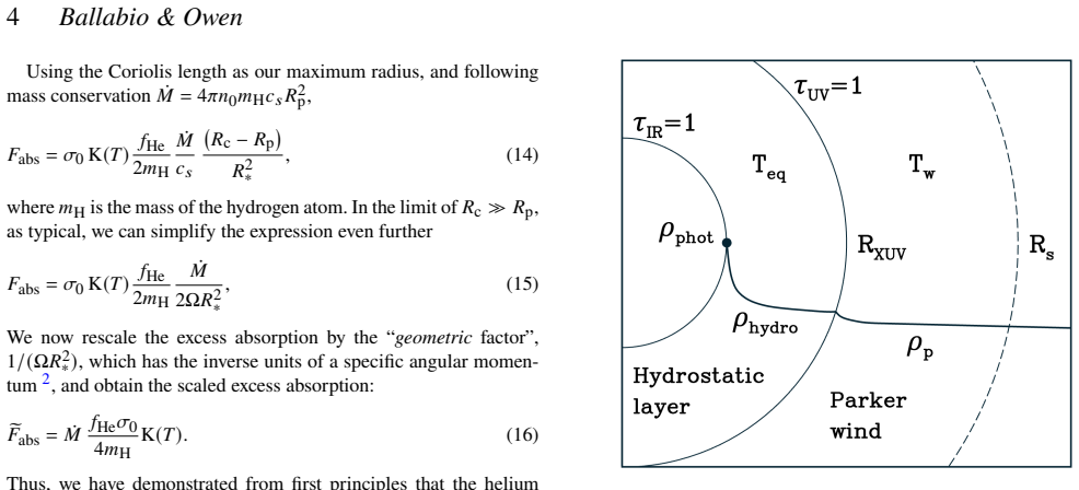
Summary. The paper develops a theoretical framework for interpreting helium 10830 Å triplet transit absorption from escaping exoplanet atmospheres. In Section 2 the authors derive an analytic scaling law, Eq. (16), claiming that a suitably scaled excess absorption is linearly proportional to the atmospheric mass-loss rate, with a temperature-dependent coefficient K(T). In Section 3 they construct a 1D two-layer atmosphere model that couples an isothermal Parker wind to an energy-limited mass-loss rate, self-consistently linking outflow temperature and mass-loss rate. They apply the model to grids of Sub-Neptunes, Neptunes, and Jupiters around a range of stellar types and orbital separations, examining correlations between the scaled equivalent width and mass-loss rate, XEUV flux, and the XEUV-to-FUV flux ratio. They also propose an observational pipeline to infer mass-loss rates from measured equivalent widths and line FWHMs.
Significance. If the central scaling law is quantitatively correct, it would establish helium absorption as a direct and practical probe of exoplanet mass-loss rates, complementing Ly-α observations that are mostly sensitive to the outflow sound speed. The paper's strengths include a first-principles analytic derivation, a numerical model that self-consistently links temperature and mass-loss rate without fitting to observations, and falsifiable predictions such as the correlation with the XEUV-to-FUV flux ratio and the suppression of helium signals around G/F stars. The parameter choices are drawn from prior literature rather than tuned to observations, which is appropriate for a theoretical study. However, the paper does not yet demonstrate that the analytic coefficient in Eq. (16) accurately reproduces the numerical model, and the strong 'direct measure' claim needs qualification given the scatter seen in the population models.
major comments (3)
- [Section 2, Eqs. (14)-(16)] The central linear scaling law is derived using three approximations that are not checked against the numerical model of Section 3: (i) the substitution Mdot = 4π n0 mH cs Rp^2 assumes v(Rp) ≈ cs, whereas a Parker wind has v(Rp) < cs for planets with the sonic point outside the base; (ii) passing from Eq. (14) to Eq. (15) drops Rp relative to the Coriolis radius Rc, an approximation that is poor for close-in Jupiter-radius planets where Rc/Rp can be of order unity; and (iii) K(T) in Eq. (9) neglects triplet photoionization, which Appendix B shows becomes important at large radii for FUV-strong stellar spectra. The manuscript never performs a direct parity check between eF_abs from the numerical model and Eq. (16). Please add such a comparison across the full parameter grid, quantifying the error introduced by each approximation. Without this check, the claim that helium absorption can be used as a direct measure of the mass-loss rate is not demonstrated.
- [Section 4.2, Figure 8] The statement in Section 2 that helium absorption 'can be used as a direct measure of the mass-loss rate' is difficult to reconcile with the finding in Section 4.2 that 'We do not find a clear correlation between the mass-loss rate and the equivalent width' once stellar spectral variability is included. The proportionality in Eq. (16) holds only for fixed temperature, geometry, and atomic parameters. The paper should specify the observational conditions (e.g., after measuring the line FWHM and adopting known stellar properties) under which the scaling becomes usable, and should quantify the residual scatter that remains in the scaled relation across the population.
- [Section 4.4, Figure 11] The proposed pipeline to determine mass-loss rates from XEUV fluxes relies on the energy-limited formula with a constant efficiency ε = 0.1, imposed at Eq. (30). Although Section 4.5 acknowledges that numerically determined efficiency factors could replace this, the inference of Mdot in Section 4.4 inherits this assumption without an uncertainty estimate. The authors should either justify ε = 0.1 for the specific parameter grid or propagate plausible variations in ε into the inferred mass-loss rates to demonstrate the robustness of the method.
minor comments (6)
- [Abstract and Section 1] The abstract states helium has been observed in '≳20 exoplanets', while Section 1 says 'more than ten confirmed detections'; please harmonize these numbers.
- [Section 2, Eq. (7)] The definition of τ1 in Eq. (7) is incomplete; please specify that it is the optical depth to helium-ionizing photons evaluated with the flux-averaged cross section introduced in Eq. (6).
- [Section 4.2, Eq. (43)] The detection-limit expression EW ≈ 3σ_noise Δλ × FWHM mixes per-pixel noise with the number of resolution elements without derivation; please clarify how many spectral pixels contribute to the equivalent width measurement.
- [References] The reference list contains 'Dos Santos et al. 2022b' with the same page range as 'Dos Santos et al. 2022a'; please verify the citation and page numbers.
- [Figures] Several figures (e.g., Figures 5 and 8) appear to lack axis labels or colorbar labels in the manuscript version; ensure all panels have complete labels and legends.
- [Throughout] There are typographical errors such as 'know asthe' in Section 1 and 'logarthimically' in Section 2; a careful proofread is needed.
Circularity Check
No significant circularity: the Eq. (16) scaling is derived from mass conservation and the optical depth integral, not fitted; the numerical model provides an independent consistency check.
full rationale
The central claim, that the scaled helium excess absorption eF_abs is proportional to the mass-loss rate Mdot times K(T), is obtained by explicit derivation from the optical depth integral (Eq. 8), the definition of excess absorption (Eq. 11), mass conservation (Mdot = 4π r^2 ρ v), and the Coriolis radius (Eq. 13). No parameter is fitted to observations to produce Eq. 16; the coefficient is fixed by atomic constants and the helium fraction. The numerical model in Section 3 solves a more complete set of level-population equations (Eqs. 38-40), so Figure 5 is a genuine test of the analytic scaling against a more detailed calculation, not a re-statement of the input. The assumption of energy-limited mass loss (Eq. 28) with ε = 0.1 is adopted from the literature, and Section 4.5 explicitly states it could be replaced by numerically determined efficiencies; this is a modeling assumption, not a fitted parameter renamed as a prediction. The self-citations to Owen & Schlichting (2024) and Schulik & Owen (2024) provide the two-layer Parker-wind framework and atomic transitions, but the scaling law is re-derived here from first principles and does not rest on those papers as a uniqueness theorem. Appendix B and Section 4.5 acknowledge limitations (triplet photoionization for FUV-strong stars, efficiency uncertainty) that affect accuracy but do not make the derivation circular.
Assumptions & free parameters
free parameters (6)
- Energy-limited efficiency epsilon =
0.1
- Bond albedo A_B =
0.3
- IR opacity kappa_IR =
10^-2 cm^2/g
- Helium fraction fHe =
0.1 (10%)
- Outer boundary R_out =
Coriolis radius R_c = c_s/(2 Omega)
- Temperature cap at 10^4 K =
10^4 K
assumptions (6)
- domain assumption The outflow is spherically symmetric and isothermal (T = constant) and follows the Parker wind solution.
- domain assumption The atmosphere is hydrogen-dominated (90% H, 10% He) with no significant fractionation.
- ad hoc to paper The energy-limited mass-loss formula with constant efficiency epsilon = 0.1 is valid.
- ad hoc to paper Statistical equilibrium for the helium triplet population (Eq. 5) holds for detectable signals.
- ad hoc to paper The outflow is truncated at the Coriolis radius R_c = c_s/(2 Omega).
- domain assumption The transit geometry is spherically symmetric and the planet is tidally locked with Omega equal to the orbital angular velocity.
Cite this review
Pith. "Pith review of Understanding what helium absorption tells us about atmospheric escape from exoplanets." pith.science (2026). https://pith.science/paper/DFMXP7BD
@misc{pith2026250106149,
  author       = {Pith},
  title        = {Pith review of: Understanding what helium absorption tells us about atmospheric escape from exoplanets},
  year         = {2026},
  howpublished = {\url{https://pith.science/paper/DFMXP7BD}},
  note         = {Machine review of arXiv:2501.06149}
}
abstract
Atmospheric escape is now considered the major contributing factor in shaping the demographic of detected exoplanets. However, inferences about the exoplanet populations strongly depend on the accuracy of the models. Direct observational tests of atmospheric models are still in their infancy. Helium escape from planetary atmospheres has rapidly become the primary observational probe, already observed in $\gtrsim$20 exoplanets. Grounding our understanding in the basic physics of atmospheric escape, we present a new theoretical model to predict the excess absorption from the helium absorption line. We constrain the atmosphere properties, such as mass-loss rates and outflow temperatures, by implementing a Parker wind solution with an energy limited evaporating outflow. Importantly, we self-consistently link the mass-loss rates and outflow temperatures, which are critical to understanding helium absorption as the triplet-level population is typically exponentially sensitive to temperature. Furthermore, helium absorption is typically optically thin and the absorption is dominated far from the planet. Therefore, the absorption depth is not a measure of the size of the helium outflow. Our results indicate that for planets with a detectable signal, typically the helium triplet population in the atmosphere rapidly approaches a statistical equilibrium between populations by recombination and depopulation caused by electron collisions. We suggest that excess helium absorption can be quantified by a scaled equivalent width, which is positively correlated with the mass loss rate. We also show that the helium absorption scales with incident radiation, particularly with the XEUV to FUV flux ratios.
Figures


Figures from the paper (8 more)


Forward citations
Cited by 1 Pith paper
-
A Self-Consistent 3D Hydrodynamic Model for Helium Transit Signatures in Evaporating Hot Jupiters
A 3D hydrodynamic model with self-consistent hydrogen-helium chemistry shows stellar winds compress escaping hot-Jupiter atmospheres and suppress the 1083 nm helium triplet signal, while a young star's strong XUV flux...
Reference graph
Works this paper leans on
-
[1]
write newline
" write newline "" before.all 'output.state := FUNCTION fin.entry write newline FUNCTION new.block output.state before.all = 'skip after.block 'output.state := if FUNCTION new.sentence output.state after.block = 'skip output.state before.all = 'skip after.sentence 'output.state := if if FUNCTION not #0 #1 if FUNCTION and 'skip pop #0 if FUNCTION or pop #1...
-
[2]
Alam M. K., et al., 2024, @doi [ ] 10.3847/1538-3881/ad50d4 , https://ui.adsabs.harvard.edu/abs/2024AJ....168..102A 168, 102
-
[3]
Allan A. P., Vidotto A. A., Villarreal D'Angelo C., Dos Santos L. A., Driessen F. A., 2024, @doi [ ] 10.1093/mnras/stad3432 , https://ui.adsabs.harvard.edu/abs/2024MNRAS.527.4657A 527, 4657
-
[4]
Allart R., et al., 2018, @doi [Science] 10.1126/science.aat5879 , https://ui.adsabs.harvard.edu/abs/2018Sci...362.1384A 362, 1384
-
[5]
Alonso-Floriano F. J., et al., 2019, @doi [ ] 10.1051/0004-6361/201935979 , https://ui.adsabs.harvard.edu/abs/2019A&A...629A.110A 629, A110
-
[6]
Baraffe I., Selsis F., Chabrier G., Barman T. S., Allard F., Hauschildt P. H., Lammer H., 2004, @doi [ ] 10.1051/0004-6361:20040129 , https://ui.adsabs.harvard.edu/abs/2004A&A...419L..13B 419, L13
-
[7]
S., Selsis F., Allard F., Hauschildt P
Baraffe I., Chabrier G., Barman T. S., Selsis F., Allard F., Hauschildt P. H., 2005, @doi [ ] 10.1051/0004-6361:200500123 , https://ui.adsabs.harvard.edu/abs/2005A&A...436L..47B 436, L47
-
[8]
Benneke B., et al., 2024, @doi [arXiv e-prints] 10.48550/arXiv.2403.03325 , https://ui.adsabs.harvard.edu/abs/2024arXiv240303325B p. arXiv:2403.03325
Show all 86 references
-
[9]
Biassoni F., Caldiroli A., Gallo E., Haardt F., Spinelli R., Borsa F., 2024, @doi [ ] 10.1051/0004-6361/202347517 , https://ui.adsabs.harvard.edu/abs/2024A&A...682A.115B 682, A115
2024 doi
-
[10]
A., 2016, @doi [ ] 10.3847/0004-637X/831/2/180 , https://ui.adsabs.harvard.edu/abs/2016ApJ...831..180C 831, 180
Chen H., Rogers L. A., 2016, @doi [ ] 10.3847/0004-637X/831/2/180 , https://ui.adsabs.harvard.edu/abs/2016ApJ...831..180C 831, 180
2016 doi
-
[11]
A., 2023, in Vidotto A
Dos Santos L. A., 2023, in Vidotto A. A., Fossati L., Vink J. S., eds, IAU Symposium Vol. 370, Winds of Stars and Exoplanets. pp 56--71 ( @eprint arXiv 2211.16243 ), @doi 10.1017/S1743921322004239
2023 arXiv
-
[13]
A., et al., 2022b, @doi [ ] 10.1051/0004-6361/202142038 , https://ui.adsabs.harvard.edu/abs/2022A&A...659A..62D 659, A62
Dos Santos L. A., et al., 2022b, @doi [ ] 10.1051/0004-6361/202142038 , https://ui.adsabs.harvard.edu/abs/2022A&A...659A..62D 659, A62
-
[14]
J., 2005, @doi [ ] 10.1111/j.1365-2966.2005.09587.x , https://ui.adsabs.harvard.edu/abs/2005MNRAS.364..649F 364, 649
Fortney J. J., 2005, @doi [ ] 10.1111/j.1365-2966.2005.09587.x , https://ui.adsabs.harvard.edu/abs/2005MNRAS.364..649F 364, 649
2005
-
[15]
France K., et al., 2016, @doi [ ] 10.3847/0004-637X/820/2/89 , https://ui.adsabs.harvard.edu/abs/2016ApJ...820...89F 820, 89
2016 doi
-
[16]
S., Lustig-Yaeger J., Fortney J
Freedman R. S., Lustig-Yaeger J., Fortney J. J., Lupu R. E., Marley M. S., Lodders K., 2014, @doi [ ] 10.1088/0067-0049/214/2/25 , https://ui.adsabs.harvard.edu/abs/2014ApJS..214...25F 214, 25
2014 doi
-
[17]
J., Petigura E
Fulton B. J., Petigura E. A., 2018, @doi [ ] 10.3847/1538-3881/aae828 , https://ui.adsabs.harvard.edu/abs/2018AJ....156..264F 156, 264
2018 doi
-
[18]
J., et al., 2017, @doi [ ] 10.3847/1538-3881/aa80eb , https://ui.adsabs.harvard.edu/abs/2017AJ....154..109F 154, 109
Fulton B. J., et al., 2017, @doi [ ] 10.3847/1538-3881/aa80eb , https://ui.adsabs.harvard.edu/abs/2017AJ....154..109F 154, 109
2017 doi
-
[19]
Garc \' a Mu \ n oz A., 2007, @doi [ ] 10.1016/j.pss.2007.03.007 , https://ui.adsabs.harvard.edu/abs/2007P&SS...55.1426G 55, 1426
2007 doi
-
[20]
E., Sari R., 2018, @doi [ ] 10.1093/mnras/sty290 , https://ui.adsabs.harvard.edu/abs/2018MNRAS.476..759G 476, 759
Ginzburg S., Schlichting H. E., Sari R., 2018, @doi [ ] 10.1093/mnras/sty290 , https://ui.adsabs.harvard.edu/abs/2018MNRAS.476..759G 476, 759
2018 doi
-
[21]
Guillot T., 2010, @doi [ ] 10.1051/0004-6361/200913396 , https://ui.adsabs.harvard.edu/abs/2010A&A...520A..27G 520, A27
2010 doi
-
[22]
Gully-Santiago M., et al., 2024, @doi [ ] 10.3847/1538-3881/ad1ee8 , https://ui.adsabs.harvard.edu/abs/2024AJ....167..142G 167, 142
2024 doi
-
[23]
E., 2019, @doi [ ] 10.1093/mnras/stz1230 , https://ui.adsabs.harvard.edu/abs/2019MNRAS.487...24G 487, 24
Gupta A., Schlichting H. E., 2019, @doi [ ] 10.1093/mnras/stz1230 , https://ui.adsabs.harvard.edu/abs/2019MNRAS.487...24G 487, 24
2019 doi
-
[24]
E., 2020, @doi [ ] 10.1093/mnras/staa315 , https://ui.adsabs.harvard.edu/abs/2020MNRAS.493..792G 493, 792
Gupta A., Schlichting H. E., 2020, @doi [ ] 10.1093/mnras/staa315 , https://ui.adsabs.harvard.edu/abs/2020MNRAS.493..792G 493, 792
2020 doi
-
[25]
E., 2021, @doi [ ] 10.1093/mnras/stab1128 , https://ui.adsabs.harvard.edu/abs/2021MNRAS.504.4634G 504, 4634
Gupta A., Schlichting H. E., 2021, @doi [ ] 10.1093/mnras/stab1128 , https://ui.adsabs.harvard.edu/abs/2021MNRAS.504.4634G 504, 4634
2021 doi
-
[26]
E., 2022, @doi [ ] 10.1093/mnras/stac2488 , https://ui.adsabs.harvard.edu/abs/2022MNRAS.516.4585G 516, 4585
Gupta A., Nicholson L., Schlichting H. E., 2022, @doi [ ] 10.1093/mnras/stac2488 , https://ui.adsabs.harvard.edu/abs/2022MNRAS.516.4585G 516, 4585
2022 doi
-
[27]
Holmberg M., Madhusudhan N., 2024, @doi [ ] 10.1051/0004-6361/202348238 , https://ui.adsabs.harvard.edu/abs/2024A&A...683L...2H 683, L2
2024 doi
-
[29]
K., L \'o pez-Morales M., Zeng L., 2020, @doi [ ] 10.3847/1538-3881/ab6e66 , https://ui.adsabs.harvard.edu/abs/2020AJ....159..115K 159, 115
Kirk J., Alam M. K., L \'o pez-Morales M., Zeng L., 2020, @doi [ ] 10.3847/1538-3881/ab6e66 , https://ui.adsabs.harvard.edu/abs/2020AJ....159..115K 159, 115
2020 doi
-
[30]
A., L \'o pez-Morales M., Alam M
Kirk J., Dos Santos L. A., L \'o pez-Morales M., Alam M. K., Oklop c i \'c A., MacLeod M., Zeng L., Zhou G., 2022, @doi [ ] 10.3847/1538-3881/ac722f , https://ui.adsabs.harvard.edu/abs/2022AJ....164...24K 164, 24
2022 doi
-
[31]
T., Yelle R
Koskinen T. T., Yelle R. V., Lavvas P., Lewis N. K., 2010, @doi [ ] 10.1088/0004-637X/723/1/116 , https://ui.adsabs.harvard.edu/abs/2010ApJ...723..116K 723, 116
2010 doi
-
[32]
Lamers H. J. G. L. M., Cassinelli J. P., 1999, Introduction to Stellar Winds
1999
-
[33]
F., Bauer S
Lammer H., Selsis F., Ribas I., Guinan E. F., Bauer S. J., Weiss W. W., 2003, @doi [ ] 10.1086/380815 , https://ui.adsabs.harvard.edu/abs/2003ApJ...598L.121L 598, L121
2003 doi
-
[34]
Lamp \'o n M., et al., 2020, @doi [ ] 10.1051/0004-6361/201937175 , https://ui.adsabs.harvard.edu/abs/2020A&A...636A..13L 636, A13
2020 doi
-
[35]
Lecavelier Des Etangs A., 2007, @doi [ ] 10.1051/0004-6361:20065014 , https://ui.adsabs.harvard.edu/abs/2007A&A...461.1185L 461, 1185
2007 doi
-
[36]
C., Oklop c i \'c A., MacLeod M., 2022, @doi [ ] 10.1051/0004-6361/202243830 , https://ui.adsabs.harvard.edu/abs/2022A&A...667A..54L 667, A54
Linssen D. C., Oklop c i \'c A., MacLeod M., 2022, @doi [ ] 10.1051/0004-6361/202243830 , https://ui.adsabs.harvard.edu/abs/2022A&A...667A..54L 667, A54
2022 doi
- [37]
-
[38]
Linssen D., Shih J., MacLeod M., Oklop c i \'c A., 2024b, @doi [ ] 10.1051/0004-6361/202450240 , https://ui.adsabs.harvard.edu/abs/2024A&A...688A..43L 688, A43
-
[39]
D., Fortney J
Lopez E. D., Fortney J. J., 2013, @doi [ ] 10.1088/0004-637X/776/1/2 , https://ui.adsabs.harvard.edu/abs/2013ApJ...776....2L 776, 2
2013 doi
-
[40]
D., Fortney J
Lopez E. D., Fortney J. J., Miller N., 2012, @doi [ ] 10.1088/0004-637X/761/1/59 , https://ui.adsabs.harvard.edu/abs/2012ApJ...761...59L 761, 59
2012 doi
-
[41]
Loyd R. O. P., et al., 2016, @doi [ ] 10.3847/0004-637X/824/2/102 , https://ui.adsabs.harvard.edu/abs/2016ApJ...824..102L 824, 102
2016 doi
-
[42]
S., et al., 2016, @doi [Nature Communications] 10.1038/ncomms11201 , https://ui.adsabs.harvard.edu/abs/2016NatCo...711201L 7, 11201
Lundkvist M. S., et al., 2016, @doi [Nature Communications] 10.1038/ncomms11201 , https://ui.adsabs.harvard.edu/abs/2016NatCo...711201L 7, 11201
2016 doi
-
[43]
MacLeod M., Oklop c i \'c A., 2022, @doi [ ] 10.3847/1538-4357/ac46ce , https://ui.adsabs.harvard.edu/abs/2022ApJ...926..226M 926, 226
2022 doi
-
[44]
Mazeh T., Holczer T., Faigler S., 2016, @doi [ ] 10.1051/0004-6361/201528065 , https://ui.adsabs.harvard.edu/abs/2016A&A...589A..75M 589, A75
2016 doi
-
[45]
A., Kratter K., Krumholz M
McCann J., Murray-Clay R. A., Kratter K., Krumholz M. R., 2019, @doi [ ] 10.3847/1538-4357/ab05b8 , https://ui.adsabs.harvard.edu/abs/2019ApJ...873...89M 873, 89
2019 doi
- [46]
- [47]
-
[48]
A., Chiang E
Murray-Clay R. A., Chiang E. I., Murray N., 2009, @doi [ ] 10.1088/0004-637X/693/1/23 , https://ui.adsabs.harvard.edu/abs/2009ApJ...693...23M 693, 23
2009 doi
-
[49]
V., Zhang Z., 2024, @doi [arXiv e-prints] 10.48550/arXiv.2410.19381 , https://ui.adsabs.harvard.edu/abs/2024arXiv241019381N p
Nail F., MacLeod M., Oklop c i \'c A., Gully-Santiago M., Morley C. V., Zhang Z., 2024, @doi [arXiv e-prints] 10.48550/arXiv.2410.19381 , https://ui.adsabs.harvard.edu/abs/2024arXiv241019381N p. arXiv:2410.19381
-
[50]
Nortmann L., et al., 2018, @doi [Science] 10.1126/science.aat5348 , https://ui.adsabs.harvard.edu/abs/2018Sci...362.1388N 362, 1388
2018 doi
-
[51]
Oklop c i \'c A., 2019, @doi [ ] 10.3847/1538-4357/ab2f7f , https://ui.adsabs.harvard.edu/abs/2019ApJ...881..133O 881, 133
2019 doi
-
[52]
M., 2018, @doi [ ] 10.3847/2041-8213/aaada9 , https://ui.adsabs.harvard.edu/abs/2018ApJ...855L..11O 855, L11
Oklop c i \'c A., Hirata C. M., 2018, @doi [ ] 10.3847/2041-8213/aaada9 , https://ui.adsabs.harvard.edu/abs/2018ApJ...855L..11O 855, L11
2018 doi
-
[53]
M., 2020, @doi [ ] 10.3847/1538-4357/ab67c6 , https://ui.adsabs.harvard.edu/abs/2020ApJ...890...88O 890, 88
Oklop c i \'c A., Silva M., Montero-Camacho P., Hirata C. M., 2020, @doi [ ] 10.3847/1538-4357/ab67c6 , https://ui.adsabs.harvard.edu/abs/2020ApJ...890...88O 890, 88
2020 doi
- [54]
-
[55]
E., 2019, @doi [Annual Review of Earth and Planetary Sciences] 10.1146/annurev-earth-053018-060246 , https://ui.adsabs.harvard.edu/abs/2019AREPS..47...67O 47, 67
Owen J. E., 2019, @doi [Annual Review of Earth and Planetary Sciences] 10.1146/annurev-earth-053018-060246 , https://ui.adsabs.harvard.edu/abs/2019AREPS..47...67O 47, 67
2019 doi
-
[56]
E., Alvarez M
Owen J. E., Alvarez M. A., 2016, @doi [ ] 10.3847/0004-637X/816/1/34 , https://ui.adsabs.harvard.edu/abs/2016ApJ...816...34O 816, 34
2016 doi
-
[57]
E., Jackson A
Owen J. E., Jackson A. P., 2012, @doi [ ] 10.1111/j.1365-2966.2012.21481.x , http://adsabs.harvard.edu/abs/2012MNRAS.425.2931O 425, 2931
2012
-
[58]
E., Lai D., 2018, @doi [ ] 10.1093/mnras/sty1760 , https://ui.adsabs.harvard.edu/abs/2018MNRAS.479.5012O 479, 5012
Owen J. E., Lai D., 2018, @doi [ ] 10.1093/mnras/sty1760 , https://ui.adsabs.harvard.edu/abs/2018MNRAS.479.5012O 479, 5012
2018 doi
-
[59]
E., Schlichting H
Owen J. E., Schlichting H. E., 2024, @doi [ ] 10.1093/mnras/stad3972 , https://ui.adsabs.harvard.edu/abs/2024MNRAS.528.1615O 528, 1615
2024 doi
-
[60]
E., Wu Y., 2013, @doi [ ] 10.1088/0004-637X/775/2/105 , https://ui.adsabs.harvard.edu/abs/2013ApJ...775..105O 775, 105
Owen J. E., Wu Y., 2013, @doi [ ] 10.1088/0004-637X/775/2/105 , https://ui.adsabs.harvard.edu/abs/2013ApJ...775..105O 775, 105
2013 doi
-
[61]
E., Wu Y., 2017, @doi [ ] 10.3847/1538-4357/aa890a , http://adsabs.harvard.edu/abs/2017ApJ...847...29O 847, 29
Owen J. E., Wu Y., 2017, @doi [ ] 10.3847/1538-4357/aa890a , http://adsabs.harvard.edu/abs/2017ApJ...847...29O 847, 29
2017 doi
-
[62]
E., et al., 2023, @doi [ ] 10.1093/mnras/stac3414 , https://ui.adsabs.harvard.edu/abs/2023MNRAS.518.4357O 518, 4357
Owen J. E., et al., 2023, @doi [ ] 10.1093/mnras/stac3414 , https://ui.adsabs.harvard.edu/abs/2023MNRAS.518.4357O 518, 4357
2023 doi
-
[63]
N., 1958, @doi [ ] 10.1086/146579 , https://ui.adsabs.harvard.edu/abs/1958ApJ...128..664P 128, 664
Parker E. N., 1958, @doi [ ] 10.1086/146579 , https://ui.adsabs.harvard.edu/abs/1958ApJ...128..664P 128, 664
1958 doi
-
[64]
Poppenhaeger K., 2022, @doi [ ] 10.1093/mnras/stac507 , https://ui.adsabs.harvard.edu/abs/2022MNRAS.512.1751P 512, 1751
2022 doi
-
[65]
E., et al., 2021, @doi [ ] 10.3847/1538-3881/ac126f , https://ui.adsabs.harvard.edu/abs/2021AJ....162..116R 162, 116
Rockcliffe K. E., et al., 2021, @doi [ ] 10.3847/1538-3881/ac126f , https://ui.adsabs.harvard.edu/abs/2021AJ....162..116R 162, 116
2021 doi
-
[66]
G., Owen J
Rogers J. G., Owen J. E., 2021, @doi [ ] 10.1093/mnras/stab529 , https://ui.adsabs.harvard.edu/abs/2021MNRAS.503.1526R 503, 1526
2021 doi
-
[67]
G., Schlichting H
Rogers J. G., Schlichting H. E., Owen J. E., 2023, @doi [ ] 10.3847/2041-8213/acc86f , https://ui.adsabs.harvard.edu/abs/2023ApJ...947L..19R 947, L19
2023 doi
-
[68]
G., Owen J
Rogers J. G., Owen J. E., Schlichting H. E., 2024, @doi [ ] 10.1093/mnras/stae563 , https://ui.adsabs.harvard.edu/abs/2024MNRAS.529.2716R 529, 2716
2024 doi
-
[69]
C., Schmitt J
Salz M., Czesla S., Schneider P. C., Schmitt J. H. M. M., 2016, @doi [ ] 10.1051/0004-6361/201526109 , https://ui.adsabs.harvard.edu/abs/2016A&A...586A..75S 586, A75
2016 doi
-
[70]
E., Loyd R
Schreyer E., Owen J. E., Loyd R. O. P., Murray-Clay R., 2024a, @doi [ ] 10.1093/mnras/stae1976 , https://ui.adsabs.harvard.edu/abs/2024MNRAS.tmp.1934S
-
[71]
E., Spake J
Schreyer E., Owen J. E., Spake J. J., Bahroloom Z., Di Giampasquale S., 2024b, @doi [ ] 10.1093/mnras/stad3528 , https://ui.adsabs.harvard.edu/abs/2024MNRAS.527.5117S 527, 5117
-
[72]
A., 2023, @doi [ ] 10.1093/mnras/stad1251 , https://ui.adsabs.harvard.edu/abs/2023MNRAS.523..286S 523, 286
Schulik M., Booth R. A., 2023, @doi [ ] 10.1093/mnras/stad1251 , https://ui.adsabs.harvard.edu/abs/2023MNRAS.523..286S 523, 286
2023 doi
- [73]
-
[74]
D., 2000, @doi [ ] 10.1086/309088 , https://ui.adsabs.harvard.edu/abs/2000ApJ...537..916S 537, 916
Seager S., Sasselov D. D., 2000, @doi [ ] 10.1086/309088 , https://ui.adsabs.harvard.edu/abs/2000ApJ...537..916S 537, 916
2000 doi
-
[75]
J., et al., 2018, @doi [ ] 10.1038/s41586-018-0067-5 , https://ui.adsabs.harvard.edu/abs/2018Natur.557...68S 557, 68
Spake J. J., et al., 2018, @doi [ ] 10.1038/s41586-018-0067-5 , https://ui.adsabs.harvard.edu/abs/2018Natur.557...68S 557, 68
2018 doi
-
[77]
J., Oklop c i \'c A., Hillenbrand L
Spake J. J., Oklop c i \'c A., Hillenbrand L. A., 2021b, @doi [ ] 10.3847/1538-3881/ac178a , https://ui.adsabs.harvard.edu/abs/2021AJ....162..284S 162, 284
-
[78]
A., Oklop c i \'c A., David T
Tyler D., Petigura E. A., Oklop c i \'c A., David T. J., 2024, @doi [ ] 10.3847/1538-4357/ad11d0 , https://ui.adsabs.harvard.edu/abs/2024ApJ...960..123T 960, 123
2024 doi
-
[79]
S., Kjeldsen H., Owen J
Van Eylen V., Agentoft C., Lundkvist M. S., Kjeldsen H., Owen J. E., Fulton B. J., Petigura E., Snellen I., 2018, @doi [ ] 10.1093/mnras/sty1783 , https://ui.adsabs.harvard.edu/abs/2018MNRAS.479.4786V 479, 4786
2018 doi
-
[80]
M., Ballester G
Vidal-Madjar A., Lecavelier des Etangs A., D \'e sert J. M., Ballester G. E., Ferlet R., H \'e brard G., Mayor M., 2003, @doi [ ] 10.1038/nature01448 , https://ui.adsabs.harvard.edu/abs/2003Natur.422..143V 422, 143
2003 doi
-
[81]
Virtanen P., et al., 2020, @doi [Nature Methods] 10.1038/s41592-019-0686-2 , https://rdcu.be/b08Wh 17, 261
2020 doi
-
[82]
Vissapragada S., et al., 2020, @doi [ ] 10.3847/1538-3881/ab8e34 , https://ui.adsabs.harvard.edu/abs/2020AJ....159..278V 159, 278
2020 doi
-
[83]
Wang L., Dai F., 2021, @doi [ ] 10.3847/1538-4357/abf1ed , https://ui.adsabs.harvard.edu/abs/2021ApJ...914...99W 914, 99
2021 doi
-
[84]
V., 2004, @doi [ ] 10.1016/j.icarus.2004.02.008 , https://ui.adsabs.harvard.edu/abs/2004Icar..170..167Y 170, 167
Yelle R. V., 2004, @doi [ ] 10.1016/j.icarus.2004.02.008 , https://ui.adsabs.harvard.edu/abs/2004Icar..170..167Y 170, 167
2004 doi
-
[85]
Youngblood A., et al., 2016, @doi [ ] 10.3847/0004-637X/824/2/101 , https://ui.adsabs.harvard.edu/abs/2016ApJ...824..101Y 824, 101
2016 doi
-
[86]
Zhang M., et al., 2022, @doi [ ] 10.3847/1538-3881/ac3f3b , https://ui.adsabs.harvard.edu/abs/2022AJ....163...68Z 163, 68
2022 doi
-
[87]
Zhang Z., et al., 2023a, @doi [Science Advances] 10.1126/sciadv.adf8736 , https://ui.adsabs.harvard.edu/abs/2023SciA....9F8736Z 9, eadf8736
-
[88]
A., Dai F., Wang L., Ricker G
Zhang M., Knutson H. A., Dai F., Wang L., Ricker G. R., Schwarz R. P., Mann C., Collins K., 2023b, @doi [ ] 10.3847/1538-3881/aca75b , https://ui.adsabs.harvard.edu/abs/2023AJ....165...62Z 165, 62
-
[89]
L., Knutson H
Zhang M., Dai F., Bean J. L., Knutson H. A., Rescigno F., 2023c, @doi [ ] 10.3847/2041-8213/aced51 , https://ui.adsabs.harvard.edu/abs/2023ApJ...953L..25Z 953, L25
Reviewed August 10, 2026 · model on record in the stance chip above.
Discussion (0). Continue with ORCID to comment.