REVIEW 4 major objections 7 minor 48 references
Fokker-Planck to Callan-Symanzik: evolution of weight matrices under training
T0 review · 4 major / 7 minor · reviewed 2026-08-10 · deepseek-v4-flash
Pith's one-line read The paper argues that, during training, the probability distribution over a weight matrix's rows follows a Fokker-Planck equation whose drift is the optimizer update and whose diffusion is set by the optimizer's noise parameters.
desk verdict Per-weight-matrix Fokker-Planck is a fair idea, but the diffusion term is numerically negligible, so the one good match only validates deterministic drift. read the letter →
The pith
A machine-rendered reading of the paper's core claim, the machinery that carries it, and where it could break.
The reading
What carries the argument
The central object is the Itô equation for a single weight-matrix row and the Fokker-Planck equation it induces for the row density $P(\vec{w},t)$; the drift is identified with the ADAM weight update and the diffusion with $\mathrm{diag}(\epsilon^2\eta^2)$. The paper treats the rows of a weight matrix as independent samples from $P$, thereby turning a matrix into a probability distribution that can be visualized in the 2D latent plane of its bottleneck layers. The numerical scheme evolves $P$ through 100 sub-time-steps per epoch, feeds the same input data through matrices drawn from the evolved density, and compares the resulting output density to the real network's. Two further identities carry the physics connection: setting $V=-\log P$ converts the Fokker-Planck equation into a generalized KPZ equation for the potential, and dropping diffusion while writing $\vec{D}=\vec{G}/t$ yields the vector Callan-Symanzik equation $t\partial_t P + \vec{G}\cdot\nabla P + P\,\nabla\cdot\vec{G}=0$, whose $\beta$-function is precisely $t\,d\vec{w}/dt$.
What would settle it
Train the same autoencoder many times from the same initialization with different random seeds, then estimate, at a fixed epoch, the conditional covariance of single-step weight increments $\vec{w}_{t+1}-\vec{w}_t$ given $\vec{w}_t$; the assumed model requires this covariance to be diagonal with entries approximately $\epsilon^2\eta^2$, independent of batch size and gradient statistics. If the measured covariance deviates from this form—for instance if it scales with batch size—the Fokker-Planck equation with drift (8-9) and diffusion (12) is not the actual training dynamics, and the reported match at epoch 5 would be a coincidence of that particular setting.
Extended reading notes
Core claim
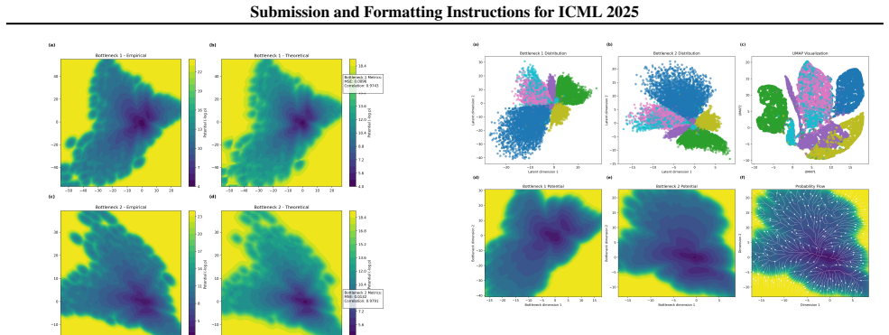
The central claim is that each weight matrix row $\vec{w}$ is driven by an Itô stochastic differential equation $d\vec{w} = \vec{D}(\vec{w},t)\,dt + \vec{\sigma}(\vec{w},t)\,d\vec{B}_t$, where the deterministic drift $\vec{D}$ is the ADAM update rule (Heaviside-gated to loss-decreasing directions) and the diffusion matrix is approximated by $\vec{\sigma}^2 \approx \mathrm{diag}(\epsilon^2\eta^2)$ with $\epsilon$ the ADAM epsilon parameter and $\eta$ the learning rate. The probability density $P(\vec{w},t)$ of the matrix's rows then obeys the Fokker-Planck equation $\partial_t P = -\nabla\cdot(\vec{D}P) + \tfrac{1}{2}\Delta(\vec{\sigma}^2 P)$, and the paper validates this by numerically integrating the equation epoch by epoch, drawing weight matrices from the evolved density, and comparing the data distribution they produce in latent space to the actual trained network's output. The validation is performed in a deliberately minimal autoencoder with two linear 2-dimensional bottleneck layers, where the theoretical and empirical latent distributions match at epoch 5 to MSE $\approx 0.012$ and Pearson correlation $\approx 0.98$. The paper's longer-range claim is that the same density evolution, when diffusion is neglected and the drift takes the form $\vec{D}=\vec{G}/t$, becomes a vector Callan-Symanzik equation whose $\beta$-function is $t\,d\vec{w}/dt$, and that the evolution of the effective potential $V=-\log P$ is a generalized Kardar-Parisi-Zhang equation.
Load-bearing premise
The argument stands on the untreated assumption that each weight-matrix row moves like the sum of a deterministic ADAM step and a random kick of fixed variance $\epsilon^2\eta^2$; the paper asserts this rather than deriving it from the training algorithm, so if the kicks do not have that form the Fokker-Planck equation does not describe training.
Editorial extensions
If this is right
- Layer-wise training can in principle be simulated by solving a Fokker-Planck PDE in the layer's width dimension, bypassing the curse of dimensionality that comes from tracking every weight in the full network.
- The terminal-time solution $P(\vec{w},T) \propto 1/|\vec{G}(\vec{w},T)|$ gives a closed-form prediction for the weight distribution whenever training reaches a stationary or scale-invariant point, and the paper suggests using it to estimate a layer's terminal training epoch after a short warm-up run.
- The Callan-Symanzik form frames the training epoch as a renormalization scale, so the layer's weight distribution at early and late times is related by a $\beta$-function flow, opening the possibility of predicting later training behavior from a brief early observation.
- Practical extensions to deeper or nonlinear architectures, such as Variational Autoencoders, are expected to require coupling separate Fokker-Planck equations across layers, which the paper leaves as the main open challenge.
Reading between the lines
- A direct test of the assumed diffusion term is to hold the optimizer and learning rate fixed while varying the minibatch size: if the noise comes from minibatch sampling, the empirical covariance of single-step weight increments should shrink with batch size, whereas the paper's $\mathrm{diag}(\epsilon^2\eta^2)$ form is batch-size independent.
- The same Fokker-Planck description might transfer from weight matrices to other parameter tensors, such as convolutional filters or attention matrices, by viewing their rows or flattened fibers as samples from a density; the bottleneck geometry would then be replaced by the appropriate row dimension of each tensor.
- Because the drift is Heaviside-gated, the equation as written is non-smooth at the point where the loss stops decreasing; analyzing that boundary may reveal when the diffusion term dominates and the density stops clustering.
- The paper's assumption that the diffusion coefficient is a constant diagonal matrix ignores possible state dependence; a modification would be to let $\sigma$ depend on the local gradient norm, which could be tested by comparing predicted versus measured latent density widths in a regime where $\epsilon$ or $\eta$ is markedly different.
Editorial analysis
A structured set of objections, weighed in public.
Referee Report
Summary. The paper proposes that the probability density of weight-matrix rows in a neural network evolves under training according to a Fokker-Planck equation. The drift is set to the ADAM update rule (Eqs. 8-9), the diffusion is chosen as σ² ~ diag(ε²η²) (Eq. 12), and the resulting PDE is solved numerically for a two-bottleneck-layer autoencoder on MNIST. The theoretical latent-space output distributions are compared with those of the actual network, reporting MSE 0.012 and Pearson correlation 0.98 at epoch 5. From the drift-dominated limit, the paper also derives a Callan-Symanzik-type equation (Eq. 17) and a Kardar-Parisi-Zhang-like potential equation (Eq. 14).
Significance. If the proposed equation were an accurate description of individual weight-matrix evolution, it would offer a tractable way to track single-layer training dynamics without the curse of dimensionality. The paper's main strengths are the concrete numerical comparison in a simple, transparent architecture, the explicit formulation of the drift from the actual optimizer, and the attempt to connect training dynamics to known physics equations. However, the significance is currently limited: the diffusion term is not derived and is numerically negligible for standard ADAM hyperparameters, the validation is a single-epoch, single-seed comparison that does not discriminate stochastic from deterministic evolution, and the Callan-Symanzik/KPZ connections are essentially formal rewritings of the continuity equation. These issues prevent the paper from establishing its central conjecture as stated.
major comments (4)
- [Sec. 2.1, Eq. (12); Sec. 4] The diffusion coefficient is specified as σ² ~ diag(ε²η²), where ε is the ADAM stability constant and η the learning rate. With typical values ε~1e-8 and η~1e-3, σ² is of order 1e-22, which is negligible compared to the drift scale. Consequently, Eq. (11) reduces to the deterministic Liouville equation ∂P/∂t = -∇·(D P), and the reported MSE=0.012 / correlation=0.98 at epoch 5 cannot distinguish the Fokker-Planck equation from the pure-drift continuity equation. The paper's own conclusion (Sec. 4) states that 'the evolution is in fact largely driven by the deterministic piece.' To support the central conjecture, the authors should either test with a noise source for which the diffusion term is non-negligible (e.g., minibatch SGD), or explicitly compare the FP solution against the pure-drift solution and show that the diffusion term changes the predicted distribution.
- [Sec. 3.2 and Sec. 3.3] The numerical procedure initializes the Fokker-Planck density from the empirical potential V_{t1} of the previous epoch, not from the initial Gaussian at epoch 0. This makes the comparison at a later epoch a one-step consistency check rather than an independent prediction of the trajectory. The text in Sec. 3.2 ('we first use the empirical 2d potential V_{t1} of the previous epoch to compute the initial condition') and Sec. 3.3 ('we simultaneously evolve the weight matrices distributions from Gaussian at epoch 0') are contradictory. Please clarify which initialization is used; if the former, the validation does not test the equation's predictive power over several epochs.
- [Sec. 3.3] The empirical validation reports a single MSE and Pearson correlation at epoch 5, with no error bars, no repeated runs, and no baseline comparisons. The later epoch-80 comparison (Fig. 9) is not given quantitative measures. To substantiate the claim that Eq. (11) describes training dynamics, the paper should report statistics over multiple random seeds and at several epochs, and should compare with a deterministic Liouville baseline and with varying diffusion coefficients.
- [Sec. 2.1.1, Eqs. (15)-(17)] The derivation of the Callan-Symanzik equation is purely formal: it assumes the drift takes the form D = G/t and then rewrites the (diffusion-less) continuity equation as Eq. (17). No justification is given for the 1/t scaling of the drift, and the identification of β = G with the usual beta function is not tied to any scale-invariance property of the training dynamics. As presented, Eq. (17) is just the Liouville equation in new notation, so the claim that the paper 'derives' the Callan-Symanzik equation is overstated. Please either provide a physical argument for the 1/t form or soften the claim.
minor comments (7)
- [Abstract and Sec. 2.1] The abstract says 'First principal derivation' and Sec. 2.1 calls Eq. (6) a 'basic first principle assumption'; an assumption is not a derivation, and the wording should be corrected to 'first-principles'.
- [Eq. (7)] The two-time correlation of the Wiener process is written with a delta function in both w and t; the standard form for Brownian motion is covariance proportional to min(t1, t2) or a delta correlation for increments, so the expression should be revised for dimensional consistency.
- [Eq. (8) vs. Eq. (9)] Eq. (8) introduces a Heaviside function that would stop updates when the loss is not decreasing, but the ADAM rule in Eq. (9) does not include such a switch, and the footnote admits the optimizer does not guarantee decreasing loss. Please clarify whether the Heaviside function is actually used in the simulations.
- [Notation, Secs. 2-3] The notation is inconsistent: w denotes a weight-matrix row in Sec. 2, while x = (x1, x2) denotes the two column dimensions in Sec. 3. Please define the mapping between w and x explicitly.
- [Eq. (28)] The MSE is computed between samples xi and yi, but the samples are not paired. Please specify how the pairing is done (e.g., sorted values or histogram bins).
- [Fig. 7] The text refers to 'figure (b) of 7' but the figure contains subfigures (a)-(d); please reference the correct subfigure.
- [Related work] The related-work section omits standard references on stochastic gradient noise and Bayesian deep learning (e.g., Mandt et al., 2017, 'Stochastic Gradient Descent as Approximate Bayesian Inference'), which are directly relevant to the assumed Ito process and the choice of the diffusion coefficient.
Circularity Check
Callan-Symanzik 'derivation' is a definitional relabeling of the continuity equation; the Fokker-Planck validation is a self-consistency check with negligible diffusion, but no load-bearing self-citation forces the central claim.
-
self definitional
[Section 2.1.1, Eqs. (15)-(17)]
"If one were to ignore the diffusion term in (11) and further rewrite on the drift function D(w,t) in a specific form: D(w,t) = G(w,t)/t (15) ... Then the evolution equation can be rewritten as G · ∇P + t ∂P/∂t + P ∇ · G = 0 (16) If we were to redefine a few coefficient functions, this can simply be written as β(w,t) · ∇P + t ∂P/∂t + n(w,t)P = 0 (17) where β(w,t) = G(w,t), n(w,t) = ∇ · G. (17) is a vector form of the Callan-Symanzik equation."
Equation (17) is obtained by defining beta := G and n := div G, so it is literally equation (16) with renamed coefficients. The paper presents this as deriving the Callan-Symanzik equation from training dynamics, but the input (16) is already the deterministic continuity equation obtained by dropping the diffusion term from (11). No new dynamical content is added; the 'derivation' is equivalent to its own input by construction. The later identification beta = t dw/dt is likewise consistent with D = beta/t by definition, so the Callan-Symanzik form is a relabeling of the drift-dominated continuity equation rather than an independent physical result.
full rationale
The central Fokker-Planck claim is not itself circular: equation (6) is explicitly stated as a 'basic first principal assumption,' equation (11) follows from it by standard Ito calculus, and the empirical comparison uses the actual ADAM update rule as the drift rather than fitting a parameter to the target output distribution. I found no load-bearing self-citation: the GenPhys citation in the introduction is motivational, and no uniqueness theorem from the authors is invoked to forbid alternatives. Two evidentiary limitations should be noted without treating them as circularity: the theoretical evolution is initialized from the previous epoch's empirical potential and advected by the actual update rule, so the reported epoch-5 match is closer to a self-consistency check than an independent long-horizon prediction; and equation (12) makes the diffusion term approximately diag(epsilon^2 eta^2), which is negligible for typical ADAM hyperparameters, so the comparison does not validate the stochastic content of the Fokker-Planck equation. These weaken the strength of the empirical support but do not make the derivation reduce to its inputs by construction. The one clear circular step is the Callan-Symanzik 'derivation,' where equation (17) is identical to equation (16) under the definitions beta = G and n = div G. Since that definitional relabeling is confined to a repackaged equation and the central conjecture retains independent content, the circularity score is 4 rather than higher.
Assumptions & free parameters
free parameters (3)
- Diffusion coefficient sigma^2 =
diag(epsilon^2 eta^2), values not reported
- Drift vector D(w,t) =
ADAM update rule gated by H(-dL/dt), values not reported
- Initial probability density P_0 =
2d Gaussian, parameters not reported
assumptions (6)
- domain assumption Each weight matrix row evolves as an Ito diffusion process with drift D and diffusion sigma.
- domain assumption The stochastic term in training can be represented by a Wiener process with zero mean and delta-function covariance.
- ad hoc to paper The diffusion coefficient is proportional to diag(epsilon^2 eta^2).
- standard math The effective potential V = -log P is well-defined and normalized to integrate to 1.
- domain assumption The 2d empirical distribution of bottleneck output data is a faithful proxy for the weight matrix distribution.
- domain assumption The ADAM update rule is a valid drift for the Ito process.
invented entities (2)
-
Effective potential V(w,t)
-
Terminal training time T
Cite this review
Pith. "Pith review of Fokker-Planck to Callan-Symanzik: evolution of weight matrices under training." pith.science (2026). https://pith.science/paper/5RN2E2SF
@misc{pith2026250109659,
  author       = {Pith},
  title        = {Pith review of: Fokker-Planck to Callan-Symanzik: evolution of weight matrices under training},
  year         = {2026},
  howpublished = {\url{https://pith.science/paper/5RN2E2SF}},
  note         = {Machine review of arXiv:2501.09659}
}
read the original abstract
The dynamical evolution of a neural network during training has been an incredibly fascinating subject of study. First principal derivation of generic evolution of variables in statistical physics systems has proved useful when used to describe training dynamics conceptually, which in practice means numerically solving equations such as Fokker-Planck equation. Simulating entire networks inevitably runs into the curse of dimensionality. In this paper, we utilize Fokker-Planck to simulate the probability density evolution of individual weight matrices in the bottleneck layers of a simple 2-bottleneck-layered auto-encoder and compare the theoretical evolutions against the empirical ones by examining the output data distributions. We also derive physically relevant partial differential equations such as Callan-Symanzik and Kardar-Parisi-Zhang equations from the dynamical equation we have.
Figures


Figures from the paper (4 more)


Reference graph
Works this paper leans on
-
[1]
write newline
" write newline "" before.all 'output.state := FUNCTION n.dashify 't := "" t empty not t #1 #1 substring "-" = t #1 #2 substring "--" = not "--" * t #2 global.max substring 't := t #1 #1 substring "-" = "-" * t #2 global.max substring 't := while if t #1 #1 substring * t #2 global.max substring 't := if while FUNCTION format.date year duplicate empty "emp...
-
[2]
Machine learning in and out of equilibrium
Adhikari, S., Kabakçıoğlu, A., Strang, A., Yuret, D., and Hinczewski, M. Machine learning in and out of equilibrium. arXiv preprint arXiv:2306.03521, 2023. URL https://arxiv.org/abs/2306.03521
work page Pith review arXiv 2023
-
[3]
S., Hu, W., Li, Z., Salakhutdinov, R., and Wang, R
Arora, S., Du, S. S., Hu, W., Li, Z., Salakhutdinov, R., and Wang, R. On exact computation with an infinitely wide neural net, 2019. URL https://arxiv.org/abs/1904.11955
arXiv 2019
-
[4]
Conditional image generation with score-based diffusion models, 2021
Batzolis, G., Stanczuk, J., Schönlieb, C.-B., and Etmann, C. Conditional image generation with score-based diffusion models, 2021. URL https://arxiv.org/abs/2111.13606
arXiv 2021
-
[5]
Bordelon , B. and Pehlevan , C. Self-consistent dynamical field theory of kernel evolution in wide neural networks . Journal of Statistical Mechanics: Theory and Experiment, 2023 0 (11): 0 114009, November 2023. doi:10.1088/1742-5468/ad01b0
-
[6]
Bordelon, B. and Pehlevan, C. Dynamics of finite width kernel and prediction fluctuations in mean field neural networks, 2023. URL https://arxiv.org/abs/2304.03408
arXiv 2023
-
[7]
Langevin algorithms for Markovian Neural Networks and Deep Stochastic control
Bras, P. and Pag \`e s, G. Langevin algorithms for markovian neural networks and deep stochastic control. arXiv preprint arXiv:2212.12018, 2022. URL https://arxiv.org/abs/2212.12018
work page Pith review arXiv 2022
-
[8]
Callan, C. G. Broken scale invariance in scalar field theory. Physical Review D, 2 0 (8): 0 1541--1547, 1970. doi:10.1103/PhysRevD.2.1541
Show all 48 references
-
[9]
and Bach, F
Chizat, L. and Bach, F. On the global convergence of gradient descent for over-parameterized models using optimal transport, 2018. URL https://arxiv.org/abs/1805.09545
2018 arXiv
-
[10]
and Rezchikov, S
Cotler, J. and Rezchikov, S. Renormalization group flow as optimal transport . Phys. Rev. D, 108 0 (2): 0 025003, 2023 a . doi:10.1103/PhysRevD.108.025003
2023 doi
-
[11]
and Rezchikov, S
Cotler, J. and Rezchikov, S. Renormalizing Diffusion Models . 8 2023 b
2023
-
[12]
S., Giampaolo, F., Rozza, G., Raissi, M., and Piccialli, F
Cuomo, S., di Cola, V. S., Giampaolo, F., Rozza, G., Raissi, M., and Piccialli, F. Scientific machine learning through physics-informed neural networks: Where we are and what's next, 2022. URL https://arxiv.org/abs/2201.05624
2022 arXiv
-
[13]
V., Kungurtsev, V., and Marecek, J
Difonzo, F. V., Kungurtsev, V., and Marecek, J. Stochastic langevin differential inclusions with applications to machine learning. arXiv preprint arXiv:2206.11533, 2022. URL https://arxiv.org/abs/2206.11533
2022 arXiv
-
[14]
Tutorial on variational autoencoders
Doersch, C. Tutorial on variational autoencoders. arXiv preprint arXiv:1606.05908, 2016. URL https://arxiv.org/abs/1606.05908
2016 arXiv
-
[15]
Erbin, H., Lahoche, V., and Samary, D. O. Renormalization in the neural network-quantum field theory correspondence, 2022. URL https://arxiv.org/abs/2212.11811
2022 arXiv
-
[16]
Disentangling feature and lazy training in deep neural networks
Geiger, M., Spigler, S., Jacot, A., and Wyart, M. Disentangling feature and lazy training in deep neural networks. Journal of Statistical Mechanics: Theory and Experiment, 2020 0 (11): 0 113301, November 2020. ISSN 1742-5468. doi:10.1088/1742-5468/abc4de. URL http://dx.doi.org...
2020 doi
-
[17]
Scalable computation of dynamic flow problems via multi-marginal graph-structured optimal transport, 2021
Haasler, I., Ringh, A., Chen, Y., and Karlsson, J. Scalable computation of dynamic flow problems via multi-marginal graph-structured optimal transport, 2021. URL https://arxiv.org/abs/2106.14485
2021 arXiv
-
[18]
Neural networks and quantum field theory
Halverson, J., Maiti, A., and Stoner, K. Neural networks and quantum field theory. Machine Learning: Science and Technology, 2 0 (3): 0 035002, April 2021. ISSN 2632-2153. doi:10.1088/2632-2153/abeca3. URL http://dx.doi.org/10.1088/2632-2153/abeca3
2021 doi
-
[19]
Hinton, G. E. and Salakhutdinov, R. R. Reducing the dimensionality of data with neural networks. Science, 313 0 (5786): 0 504--507, 2006. doi:10.1126/science.1127647. URL https://www.science.org/doi/abs/10.1126/science.1127647
2006 doi
-
[20]
Denoising diffusion probabilistic models, 2020
Ho, J., Jain, A., and Abbeel, P. Denoising diffusion probabilistic models, 2020. URL https://arxiv.org/abs/2006.11239
2020 arXiv
-
[21]
N., Klinger, M
Howard, J. N., Klinger, M. S., Maiti, A., and Stapleton, A. G. Bayesian RG Flow in Neural Network Field Theories . 5 2024
2024
-
[22]
Neural tangent kernel: Convergence and generalization in neural networks, 2020
Jacot, A., Gabriel, F., and Hongler, C. Neural tangent kernel: Convergence and generalization in neural networks, 2020. URL https://arxiv.org/abs/1806.07572
2020 arXiv
-
[23]
Dynamic scaling of growing interfaces
Kardar, M., Parisi, G., and Zhang, Y.-C. Dynamic scaling of growing interfaces. Phys. Rev. Lett., 56: 0 889--892, Mar 1986. doi:10.1103/PhysRevLett.56.889. URL https://link.aps.org/doi/10.1103/PhysRevLett.56.889
1986 doi
-
[24]
Physics-informed machine learning
Karniadakis, G., Kevrekidis, I., Lu, L., Perdikaris, P., Wang, S., and Yang, L. Physics-informed machine learning. Nature Reviews Physics, 3 0 (6): 0 422--440, June 2021. ISSN 2522-5820. doi:10.1038/s42254-021-00314-5. Publisher Copyright: 2021, Springer Nature Limited
2021 doi
-
[25]
Kingma, D. P. and Welling, M. Auto-encoding variational bayes, 2022. URL https://arxiv.org/abs/1312.6114
2022 arXiv
-
[26]
Optimal flow matching: Learning straight trajectories in just one step, 2024
Kornilov, N., Mokrov, P., Gasnikov, A., and Korotin, A. Optimal flow matching: Learning straight trajectories in just one step, 2024. URL https://arxiv.org/abs/2403.13117
2024 arXiv
-
[27]
Kunin, D., Sagastuy-Brena, J., Gillespie, L., Margalit, E., Tanaka, H., Ganguli, S., and Yamins, D. L. K. The limiting dynamics of sgd: Modified loss, phase-space oscillations, and anomalous diffusion. Neural Computation, 36 0 (1): 0 151–174, December 2023. ISSN 1530-888X. doi...
2023 doi
-
[28]
S., Bahri, Y., Novak, R., Sohl-Dickstein, J., and Pennington, J
Lee, J., Xiao, L., Schoenholz, S. S., Bahri, Y., Novak, R., Sohl-Dickstein, J., and Pennington, J. Wide neural networks of any depth evolve as linear models under gradient descent *. Journal of Statistical Mechanics: Theory and Experiment, 2020 0 (12): 0 124002, December 2020....
2020 doi
-
[29]
Accelerating convergence of score-based diffusion models, provably, 2024
Li, G., Huang, Y., Efimov, T., Wei, Y., Chi, Y., and Chen, Y. Accelerating convergence of score-based diffusion models, provably, 2024. URL https://arxiv.org/abs/2403.03852
2024 arXiv
-
[30]
Genphys: From physical processes to generative models, 2023
Liu, Z., Luo, D., Xu, Y., Jaakkola, T., and Tegmark, M. Genphys: From physical processes to generative models, 2023. URL https://arxiv.org/abs/2304.02637
2023 arXiv
-
[31]
Designing optimal networks for multicommodity transport problem
Lonardi, A., Facca, E., Putti, M., and De Bacco, C. Designing optimal networks for multicommodity transport problem. Physical Review Research, 3 0 (4), October 2021. ISSN 2643-1564. doi:10.1103/physrevresearch.3.043010. URL http://dx.doi.org/10.1103/PhysRevResearch.3.043010
2021 doi
-
[32]
and Bihlo, A
Matthews, J. and Bihlo, A. Pinnde: Physics-informed neural networks for solving differential equations, 2024. URL https://arxiv.org/abs/2408.10011
2024 arXiv
-
[33]
A mean field view of the landscape of two-layer neural networks
Mei, S., Montanari, A., and Nguyen, P.-M. A mean field view of the landscape of two-layer neural networks. Proceedings of the National Academy of Sciences, 115 0 (33), July 2018. ISSN 1091-6490. doi:10.1073/pnas.1806579115. URL http://dx.doi.org/10.1073/pnas.1806579115
2018 doi
-
[34]
Mean-field langevin dynamics and energy landscape of neural networks
Mei, S., Montanari, A., and Nguyen, P.-M. Mean-field langevin dynamics and energy landscape of neural networks. The Annals of Applied Probability, 29 0 (6): 0 3521--3562, 2019. URL https://projecteuclid.org/journals/annales-de-linstitut-henri-poincare-probabilites-et-statistiq...
2019 doi
-
[35]
and Bouchaud, J.-P
Potters, M. and Bouchaud, J.-P. A First Course in Random Matrix Theory: for Physicists, Engineers and Data Scientists. Cambridge University Press, 2020
2020
-
[36]
Raissi, M., Perdikaris, P., and Karniadakis, G. E. Physics-informed neural networks: A deep learning framework for solving forward and inverse problems involving nonlinear partial differential equations. J. Comput. Phys., 378: 0 686--707, 2019. URL https://api.semanticscholar....
2019
-
[37]
J., Mohamed, S., and Wierstra, D
Rezende, D. J., Mohamed, S., and Wierstra, D. Stochastic backpropagation and approximate inference in deep generative models. In Xing, E. P. and Jebara, T. (eds.), Proceedings of the 31st International Conference on Machine Learning, volume 32 of Proceedings of Machine Learnin...
2014
-
[38]
and Vanden‐Eijnden, E
Rotskoff, G. and Vanden‐Eijnden, E. Trainability and accuracy of artificial neural networks: An interacting particle system approach. Communications on Pure and Applied Mathematics, 75 0 (9): 0 1889–1935, July 2022. ISSN 1097-0312. doi:10.1002/cpa.22074. URL http://dx.doi.org/...
1935 doi
-
[39]
and Spiliopoulos, K
Sirignano, J. and Spiliopoulos, K. Dgm: A deep learning algorithm for solving partial differential equations. Journal of Computational Physics, 375: 0 1339–1364, December 2018. ISSN 0021-9991. doi:10.1016/j.jcp.2018.08.029. URL http://dx.doi.org/10.1016/j.jcp.2018.08.029
2018 doi
-
[40]
Maximum likelihood training of score-based diffusion models, 2021 a
Song, Y., Durkan, C., Murray, I., and Ermon, S. Maximum likelihood training of score-based diffusion models, 2021 a . URL https://arxiv.org/abs/2101.09258
2021 arXiv
-
[41]
P., Kumar, A., Ermon, S., and Poole, B
Song, Y., Sohl-Dickstein, J., Kingma, D. P., Kumar, A., Ermon, S., and Poole, B. Score-based generative modeling through stochastic differential equations, 2021 b . URL https://arxiv.org/abs/2011.13456
2021 arXiv
-
[42]
Small distance behavior in field theory and power counting
Symanzik, K. Small distance behavior in field theory and power counting. Communications in Mathematical Physics, 18: 0 227--246, 1970. doi:10.1007/BF01649434
1970 doi
-
[43]
Improving and generalizing flow-based generative models with minibatch optimal transport, 2024
Tong, A., Fatras, K., Malkin, N., Huguet, G., Zhang, Y., Rector-Brooks, J., Wolf, G., and Bengio, Y. Improving and generalizing flow-based generative models with minibatch optimal transport, 2024. URL https://arxiv.org/abs/2302.00482
2024 arXiv
-
[44]
and Teh, Y
Welling, M. and Teh, Y. W. Bayesian learning via stochastic gradient langevin dynamics. In International Conference on Machine Learning, 2011. URL https://api.semanticscholar.org/CorpusID:2178983
2011
-
[45]
and Hu, E
Yang, G. and Hu, E. J. Feature learning in infinite-width neural networks, 2022. URL https://arxiv.org/abs/2011.14522
2022 arXiv
-
[46]
and Littwin, E
Yang, G. and Littwin, E. Tensor programs iib: Architectural universality of neural tangent kernel training dynamics, 2021. URL https://arxiv.org/abs/2105.03703
2021 arXiv
-
[47]
Ye, N., Zhu, Z., and Mantiuk, R. K. Langevin dynamics with continuous tempering for training deep neural networks, 2017. URL https://arxiv.org/abs/1703.04379
2017 arXiv
-
[48]
and Huang, H
Zou, W. and Huang, H. Introduction to dynamical mean-field theory of randomly connected neural networks with bidirectionally correlated couplings. SciPost Physics Lecture Notes, February 2024. ISSN 2590-1990. doi:10.21468/scipostphyslectnotes.79. URL http://dx.doi.org/10.21468...
2024 doi
Reviewed August 10, 2026 · model on record in the stance chip above.
Discussion (0). Continue with ORCID to comment.