REVIEW 4 major objections 5 minor 1 cited by
Semiclassical Mixmaster Universe
T0 review · 4 major / 5 minor · reviewed 2026-08-10 · deepseek-v4-flash
Pith's one-line read Polymerizing the volume in the Mixmaster universe replaces the singular collapse with a sequence of asymmetric bounces and systematically lowers the maximal Lyapunov exponent relative to the classical model, with quantum matter back…
desk verdict The qualitative bounce and scalar-excitation results are solid and new, but the headline chaos-reduction claim rests on Lyapunov exponents in coordinate time over unequal intervals, with the invariant box-counting measure showing only marginal differences. read the letter →
The pith
A machine-rendered reading of the paper's core claim, the machinery that carries it, and where it could break.
The reading
What carries the argument
The central object is the polymerized (effective) Hamiltonian constraint $H^{\mathrm{eff}}_{IX} = -\frac{3}{8\lambda^2}\nu\sin^2(\lambda p_\nu) + \frac{1}{24\nu}(p_+^2+p_-^2) + \nu^{1/3}V_{IX}(\beta_+,\beta_-)$, obtained from the classical Mixmaster constraint by the replacement $p_\nu \to \sin(\lambda p_\nu)/\lambda$. This bounded-momentum replacement produces the modified Hubble rate $H_\nu^2 = \frac{3}{2}\rho_T(1-\rho_T/\rho_\mathrm{crit})$ with $\rho_\mathrm{crit}=3/(8\lambda^2)$, so the volume bounces instead of collapsing to zero. Here $V_{IX}$ is the triangular wall potential of the Mixmaster billiard. For the quantum matter cases, the scalar field enters through the expectation value $\langle\psi|\hat{H}_\phi|\psi\rangle$ in the constraint, with the state evolving by the Schr\"odinger equation, giving non-perturbative back reaction.
What would settle it
Recompute the maximal Lyapunov exponent for the effective Hamiltonians with $\lambda = 0.05$, $0.2$, and $0.5$ under the same initial data; if any of these yields an exponent close to the classical value (3.210 for vacuum or 4.4320 with matter), the claimed chaos reduction is an artifact of the chosen lattice scale rather than a robust quantum-gravity effect.
Extended reading notes
Core claim
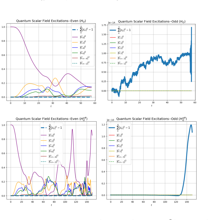
The paper's central claim is that LQG-inspired volume discreteness, implemented by the replacement $p_\nu \to \sin(\lambda p_\nu)/\lambda$ in the Bianchi IX Hamiltonian, changes the classical picture of a chaotic approach to the singularity into a bouncing dynamics with reduced chaos. In all effective-gravity models considered, the volume undergoes several small, asymmetric bounces before expanding; the anisotropies grow and fall through each bounce, more strongly when matter is present; and the maximal Lyapunov exponent is smaller than in the corresponding classical models — from $4.4320$ for classical gravity with a classical scalar field to $1.024$ for effective gravity with a quantum scalar field. With a quantum scalar field, the field state is excited out of its ground state as the bounce is approached and does not fully return to the ground state afterwards, indicating a back-reaction memory of the bounce. The paper also finds that while the Kasner sum rule is preserved and tends to unity at the classical singularity, it is constant but not unity away from the bounce and oscillates through the bounce, showing that 'matter matters' when a bounce replaces the singularity.
Load-bearing premise
The load-bearing premise is that polymerizing only the volume momentum with a hand-chosen lattice scale $\lambda = 0.1$ captures the relevant quantum gravity effects near the singularity; the number of bounces and the Lyapunov exponents depend on this scale and on leaving anisotropies and the scalar field unpolymerized.
Editorial extensions
If this is right
- The classical singularity in Bianchi IX is replaced by a finite number of asymmetric bounces; the approach to the bounce is not Kasner-like, so the classical 'matter does not matter' behavior does not extend to bouncing cosmologies.
- A quantum scalar field initially in its ground state becomes excited through the bounce and retains some excitation at late times, so quantum matter back reaction leaves a memory of the bounce.
- The maximal Lyapunov exponent drops substantially in effective gravity, from 3.210 to 0.4093 in vacuum and from 4.4320 to 1.024 with a quantum scalar field, so the bounce reduces rather than eliminates chaos.
- Because a minimum volume saturates the number of wall collisions, any singularity-replacing bounce is expected to reduce chaos, making the result not specific to polymer quantization.
- The fractal dimension of the anisotropy attractor is slightly lower for effective gravity (values in [1.72, 1.77]), consistent with reduced chaos but too close to sharply rank the models.
Reading between the lines
- The quantitative results depend on the hand-chosen lattice scale $\lambda = 0.1$; if the full theory pins $\lambda$ to the area gap, the number of bounces and Lyapunov exponents would shift, so the specific numbers in Table I should be read as predictions conditional on that scale.
- The persistence of scalar-field excitations after the bounce suggests a potential observational signature in primordial spectra, but this homogeneous model would need an inhomogeneous extension before any concrete prediction.
- The same self-consistent back-reaction scheme could be applied to Gowdy cosmologies; the authors note this would require maintaining the constraint algebra with matter expectation value terms.
- The finding that the Kasner sum oscillates through the bounce rather than staying constant indicates that the effective bounce is a genuinely non-Kasner phase, a feature that any alternative bounce mechanism should reproduce.
Editorial analysis
A structured set of objections, weighed in public.
Referee Report
Summary. The paper studies Bianchi IX (Mixmaster) cosmology with three gravitational/matter settings: classical gravity with classical or quantum scalar field, and polymerized ('effective') gravity with classical or quantum scalar field, plus the corresponding vacuum cases. The polymer model replaces the volume momentum by sin(λ p_ν)/λ in the Hamiltonian constraint, which produces bouncing evolutions. Numerically, the authors report multiple bounces, anisotropy growth through bounces, scalar field excitation during bounces, and a claimed reduction of chaos in the effective models, quantified by maximal Lyapunov exponents and box-counting fractal dimensions. Constraint and probability conservation are checked to high precision.
Significance. If the chaos-reduction claim is correct, the paper would be a useful quantitative step connecting loop-inspired discreteness to Mixmaster dynamics, and the nonperturbative quantum-scalar-field backreaction scheme is methodologically interesting. The explicit verification of Hamiltonian constraint and probability conservation in the mixed classical-quantum system is a strength, as is the clear comparative setup of six models. However, the central claim (iii) currently rests on Lyapunov exponents computed in a coordinate-time gauge for systems that are not comparable in their time intervals and that are known to have gauge-dependent chaos indicators. The supporting fractal-dimension analysis is explicitly marginal, so the main physical conclusion is not yet established.
major comments (4)
- [§III.C.1, Eq. (37), Table I] The maximal Lyapunov exponents in Table I are computed from the N=1 coordinate-time system, but the classical trajectories terminate at the singularity near t=40–55 while the effective bouncing trajectories are evolved to t=200. The limit in Eq. (37) is therefore not attained for the classical cases, making the comparison one between finite-time exponents of a singular flow and longer-time exponents of a bounded flow. Since the paper itself cites Refs. [14,15] on the inconsistency of chaos indicators under time reparametrization for constrained systems, a demonstration that the reduction persists for an invariant clock (for example, using the Kasner transition map or a deparameterization with the scalar field) is required before claim (iii) can be supported. The box-counting result in §III.C.2 varies only in [1.72,1.77] and is called marginal by the authors, so it does not independently corroborate the factor-of-several reduction.
- [§III.C.1, Table I] The entry HC = HQ = 4.4320 to four decimal places is suspicious: the classical-gravity cases with a classical versus a quantum scalar field are different dynamical systems, yet the reported maximal exponents are exactly identical. This suggests either that the observable is insensitive to the difference (which would undermine the resolution of the method) or that the numerical pipeline is not fully resolving the dynamics. No error bars, no dependence on the reorthonormalization interval, and no multi-trajectory statistics are reported, so the table cannot be evaluated quantitatively. I ask for a convergence study and uncertainty estimates for the Lyapunov exponents.
- [§III, Eq. (33)] The scalar-field Hilbert space is truncated at n=30, and the authors state that 'changing truncation level does not significantly affect our results provided the initial state is the ground state,' but no convergence data are shown. This truncation directly affects the quantum backreaction terms in the H_eff_Q equations and hence the Lyapunov exponent for that model. A truncation-level scan should be presented for the state coefficients, the expectation values entering the constraint, and the maximal Lyapunov exponent.
- [§II.A, Eq. (17), §III] The quantitative results—number of bounces, scalar excitation amplitudes, and the Lyapunov exponents—depend on the polymer scale λ=0.1 and the scalar mass m=0.01, which are chosen 'for all illustrative numerical evolutions' without a sensitivity analysis. Since λ enters the critical density ρ_crit via ρ_crit=3/8λ^2, the reported factor-of-four reduction in chaos is a function of this parameter. A λ- and m-dependence study (at least a sweep over a plausible range) is needed to turn the qualitative observation into a quantitative claim.
minor comments (5)
- [§III.C heading and reference [43]] The heading contains the typo 'Lyupanov exponents' instead of 'Lyapunov exponents', and Ref. [43] spells the author as 'Bennetin'; it should be Benettin.
- [Eq. (31)] The expression for ρ_T appears to have a dimensional inconsistency: the scalar-field term is written as (1/ν)H_ϕ inside the bracket, which gives H_ϕ/ν^2 after the overall 1/ν factor, whereas Eq. (34) defines the scalar density as H_ϕ/ν. Please correct the factor or clarify the intended definition.
- [Fig. 3 caption] The caption contains a doubled word: 'the first few and and the last few even-state excitations' should read 'the first few and the last few'.
- [Eq. (32) and surrounding text] The matching of classical initial data via φ(0)=√⟨φ^2⟩ and p_φ(0)=√⟨p_φ^2⟩ is a specific choice that is not equivalent to setting the classical variables equal to the expectation values of the quantum state; this choice should be stated explicitly as a convention and its impact on the comparison discussed.
- [Fig. 8 caption] The caption says 'We see here the results...' and 'we use the polymerized and unpolymerized counterparts for each species'; please make the caption self-contained and define 'unpolymerized' explicitly, since it refers to the classical Hamiltonian cases.
Circularity Check
No significant circularity: the bounce is a transparent model consequence and the chaos-reduction claim is an independent numerical output.
full rationale
The paper does not fit parameters and rename them as predictions. The effective Hamiltonian is obtained by the explicitly stated polymer replacement p_nu -> sin(lambda p_nu)/lambda (Eq. 17), and the paper itself notes that the bounce 'is due to this last feature' via the derived Hubble rate (Eq. 30). Presenting the bounce as a finding is a model consequence, not a circular derivation, because the replacement is not defined in terms of the bounce and the number/structure of bounces is not fixed by the input. The scalar-field excitation pattern, anisotropy behavior, and Lyapunov exponents are numerical outputs not fed back into the model; no target result is enforced by construction. Self-citations (e.g., Refs. [32], [39]) provide background and motivation rather than load-bearing uniqueness arguments. Potential concerns about Lyapunov exponent gauge dependence or comparison over unequal time intervals are validity/correctness issues, not circularity.
Assumptions & free parameters
free parameters (5)
- polymer scale lambda =
0.1
- scalar field mass m =
0.01
- initial data =
nu(0)=10, beta+(0)=-0.05, beta-(0)=0.01, p-(0)=-10, p_nu(0)=-5
- Hilbert space truncation n=30 =
30
- box-counting gray threshold =
90%
assumptions (4)
- domain assumption The Bianchi IX Hamiltonian constraint H_IX (Eq. 7) and scalar field H_phi (Eq. 6) are the correct classical description in Misner variables.
- domain assumption The polymer replacement p_nu -> sin(lambda p_nu)/lambda (Eq. 17) is the correct effective quantum gravity correction, with lambda fixed by hand.
- domain assumption The semiclassical backreaction scheme using <H_phi> and the Schrodinger equation (Eqs. 26 and 27) is a valid non-perturbative method.
- ad hoc to paper Truncating the scalar field Hilbert space at n=30 in the initial oscillator basis preserves the relevant dynamics.
Cite this review
Pith. "Pith review of Semiclassical Mixmaster Universe." pith.science (2026). https://pith.science/paper/SEY34GZJ
@misc{pith2026250114891,
  author       = {Pith},
  title        = {Pith review of: Semiclassical Mixmaster Universe},
  year         = {2026},
  howpublished = {\url{https://pith.science/paper/SEY34GZJ}},
  note         = {Machine review of arXiv:2501.14891}
}
read the original abstract
We present a semiclassical study of the Mixmaster cosmology minimally coupled to a massive scalar field in the Hamiltonian formalism, with focus on three distinct scenarios: the classical cosmology coupled to the quantized scalar field, and "effective" cosmology, with spacetime discreteness corrections, coupled to the classical scalar field, and to the quantized scalar field. We find several results: (i) the effective cosmology undergoes several small bounces before expanding, with scalar field excitations rising through the bounce; (ii) anisotropies rise and fall as the universe undergoes a bounce, a feature that is enhanced with matter; (iii) Lyapunov exponents reveal that chaos is reduced in the effective systems compared to the classical case.
Figures


Figures from the paper (5 more)


Forward citations
Cited by 1 Pith paper
-
Polymer Bianchi-I with polymer matter
In a Bianchi-I universe with polymer quantization of both geometry and a massless scalar, the matter polymer scale shifts the quantum bounce and alters volume and anisotropy evolution.
Reference graph
Works this paper leans on
-
[27]
Wilson-Ewing, Classical and Quantum Gravity 36, 195002 (2019)
E. Wilson-Ewing, Classical and Quantum Gravity 36, 195002 (2019)
work page 2019
-
[1]
Effective cosmology with classical scalar field The dynamics of the first model we consider follows from the effective constraint H eff C ≡ H eff IX + Hϕ = 0, (19) where the scalar field part of the Hamiltonian constraint remains unmodified and H eff IX is defined in eqn.(18). The equations of motions are ˙ν = {ν, H eff C } = − 3 8 ν sin(2λpν) λ , (20) ˙p...
-
[2]
Effective cosmology with quantum scalar field The second model we study uses an effective constraint where the scalar field is quantized its quantum state evolves via the time dependent Schr¨ odinger equation. This may be viewed as the canonical version of the semi- classical Einstein equation applied to cosmology, but with the polymer quantization correc...
-
[3]
An n−dimensional phase space has n such exponents
Lyapunov exponents One measure of chaos is the Lyapunov exponent: given two infinitesimally close initial data points x1(0) and x2(0) for a dynamical system, if the initial separation ξ(0) = |x2(0) − x1(0)| grows as ξ(t) ∼ ξ(0)eλt with λ >0 the system is considered to be chaotic, and λ is called the Lyapunov exponent. An n−dimensional phase space has n su...
-
[4]
One of these is the so-called box counting method computed from images of the fractal
Fractal dimension There are several methods for estimating the fractal dimension of attractor sets in phase space [16, 44]. One of these is the so-called box counting method computed from images of the fractal. For a fractal set F , the num- ber N of boxes of size ϵ it takes to cover F scales as log(N (ϵ)) = −D log(ϵ). (38) We apply this to the phase spac...
-
[5]
V. A. Belinskii and I. M. Khalatnikov, Sov. Phys. JETP 29, 911 (1969)
work page 1969
-
[6]
V. Belinski ˘ ı, E. Lifshitz, and I. M. Khalatnikov, Soviet Physics Uspekhi 13, 745 (1971)
work page 1971
-
[7]
M. P. Ryan and L. C. Shepley, Homogeneous Relativistic Cosmologies, Princeton Series in Physics (Princeton Uni- versity Press, Princeton, 1975), ISBN 978-0-691-08146-5, 069101530
work page 1975
Show all 48 references
-
[8]
C. W. Misner, Physical Review Letters 22, 1071 (1969)
1969
-
[9]
C. W. Misner, Phys. Rev. 186, 1319 (1969), URL https: //link.aps.org/doi/10.1103/PhysRev.186.1319
1969 doi
-
[11]
D. F. Chernoff and J. D. Barrow, Phys. Rev. Lett. 50, 134 (1983), URL https://link.aps.org/doi/10.1103/ PhysRevLett.50.134
1983
-
[12]
J. D. Barrow, Phys. Rev. Lett. 46, 963 (1981), URL https://link.aps.org/doi/10.1103/PhysRevLett.46. 963
1981 doi
-
[13]
Hobill, D
D. Hobill, D. Bernstein, M. Welge, and D. Simkins, Clas- sical and Quantum Gravity 8, 1155 (1991)
1991
-
[14]
A. Burd, N. Buric, and G. Ellis, General relativity and gravitation 22, 349 (1990)
1990
-
[15]
Kiefer, N
C. Kiefer, N. Kwidzinski, and W. Piechocki, The Euro- pean Physical Journal C 78, 1 (2018)
2018
-
[16]
D. Bini, C. Cherubini, A. Geralico, and R. T. Jantzen, Classical and Quantum Gravity 26, 025012 (2009)
2009
-
[17]
Andriopoulos and P
K. Andriopoulos and P. Leach, Journal of Physics A: Mathematical and Theoretical 41, 155201 (2008)
2008
-
[18]
Ferraz and G
K. Ferraz and G. Francisco, Phys. Rev. D 45, 1158 (1992), URL https://link.aps.org/doi/10. 1103/PhysRevD.45.1158
1992
-
[19]
Szydlowski and A
M. Szydlowski and A. Krawiec, Phys. Rev. D 47, 5323 (1993), URL https://link.aps.org/doi/10. 1103/PhysRevD.47.5323
1993
-
[20]
N. J. Cornish and J. J. Levin, Phys. Rev. Lett. 78, 998 (1997), URL https://link.aps.org/doi/10.1103/ PhysRevLett.78.998
1997
-
[21]
N. J. Cornish and J. J. Levin, Phys. Rev. D 55, 7489 (1997), URL https://link.aps.org/doi/10. 1103/PhysRevD.55.7489
1997
-
[22]
Imponente and G
G. Imponente and G. Montani, Phys. Rev. D 63, 103501 (2001), URL https://link.aps.org/doi/10. 1103/PhysRevD.63.103501
2001
-
[23]
Damour and M
T. Damour and M. Henneaux, Phys. Rev. Lett. 85, 920 (2000), URL https://link.aps.org/doi/10.1103/ PhysRevLett.85.920
2000
-
[24]
Ashtekar, A
A. Ashtekar, A. Henderson, and D. Sloan, Phys. Rev. D 83, 084024 (2011), URL https://link.aps.org/doi/ 10.1103/PhysRevD.83.084024
2011 doi
-
[25]
Barnich and V
G. Barnich and V. Husain, Class. Quant. Grav. 14, 1043 (1997), gr-qc/9611030
1997 arXiv
-
[26]
Wilson-Ewing, Classical and Quantum Gravity 35, 065005 (2018)
E. Wilson-Ewing, Classical and Quantum Gravity 35, 065005 (2018)
2018
-
[28]
Blackmore and E
T. Blackmore and E. Wilson-Ewing, Classical and Quan- tum Gravity 40, 215010 (2023)
2023
-
[30]
Bojowald, D
M. Bojowald, D. Brizuela, P. Calizaya Cabrera, and S. F. Uria, Phys. Rev. D 109, 044038 (2024), URL https: //link.aps.org/doi/10.1103/PhysRevD.109.044038
2024 doi
-
[31]
Bojowald, D
M. Bojowald, D. Brizuela, P. C. Cabrera, and S. F. Uria, Phys. Rev. D 108, L061501 (2023), URL https://link. aps.org/doi/10.1103/PhysRevD.108.L061501
2023 doi
-
[32]
Brizuela and S
D. Brizuela and S. F. Uria, Phys. Rev. D 106, 064051 (2022), URL https://link.aps.org/doi/10. 1103/PhysRevD.106.064051
2022
-
[33]
Husain and S
V. Husain and S. Singh, Phys. Rev. D 99, 086018 (2019), URL https://link.aps.org/doi/10.1103/PhysRevD. 99.086018
2019 doi
-
[34]
Husain and S
V. Husain and S. Singh, Phys. Rev. D 104, 124048 (2021), URL https://link.aps.org/doi/10. 1103/PhysRevD.104.124048
2021
-
[35]
Ali and V
M. Ali and V. Husain, Physical Review D 96 (2017), ISSN 2470-0029, URL http://dx.doi.org/10.1103/ PhysRevD.96.044032
2017
-
[36]
Husain and M
V. Husain and M. Muzammil, Physical Review D 109, 044063 (2024)
2024
-
[37]
H. Halvorson, Studies in History and Philosophy of Sci- ence Part B: Studies in History and Philosophy of Mod- ern Physics 35, 45–56 (2004), ISSN 1355-2198, URL http://dx.doi.org/10.1016/j.shpsb.2003.01.001
2004 doi
-
[38]
Ashtekar, S
A. Ashtekar, S. Fairhurst, and J. L. Willis, Clas- sical and Quantum Gravity 20, 1031–1061 (2003), ISSN 0264-9381, URL http://dx.doi.org/10.1088/ 0264-9381/20/6/302
2003
-
[39]
Fredenhagen and F
K. Fredenhagen and F. Reszewski, Classical and Quantum Gravity 23, 6577–6584 (2006), ISSN 1361- 6382, URL http://dx.doi.org/10.1088/0264-9381/ 23/22/028
2006 doi
-
[40]
J. M. Velhinho, Classical and Quantum Gravity 24, 3745–3758 (2007), ISSN 1361-6382, URL http://dx. doi.org/10.1088/0264-9381/24/14/013
2007 doi
- [41]
- [42]
- [43]
-
[44]
Agullo and P
I. Agullo and P. Singh, Loop quantum cosmology: A brief review (2016), 1612.01236, URL https://arxiv. org/abs/1612.01236
2016 arXiv
-
[45]
Bodendorfer, An elementary introduction to loop quantum gravity (2016), 1607.05129, URL https:// arxiv.org/abs/1607.05129
N. Bodendorfer, An elementary introduction to loop quantum gravity (2016), 1607.05129, URL https:// arxiv.org/abs/1607.05129
2016 arXiv
-
[46]
Giovannetti and G
E. Giovannetti and G. Montani, Phys. Rev. D 100, 104058 (2019), URL https://link.aps.org/doi/10. 1103/PhysRevD.100.104058
2019
-
[47]
Benettin, L
G. Benettin, L. Galgani, and J.-M. Strelcyn, Physical Review A 14, 2338 (1976)
1976
-
[48]
S. H. Strogatz, Nonlinear dynamics and chaos: with ap- plications to physics, biology, chemistry, and engineering (CRC press, 2018)
2018
-
[49]
Moriconi, G
R. Moriconi, G. Montani, and S. Capozziello, Phys. Rev. D 90, 101503 (2014), 1411.0441
2014 arXiv
- [50]
Reviewed August 10, 2026 · model on record in the stance chip above.
Discussion (0). Continue with ORCID to comment.