Predicting three-dimensional chaotic systems with four qubit quantum systems

Christoph R\"ath; Joel Steinegger

REVIEW 3 major objections 6 minor 52 references

Predicting three-dimensional chaotic systems with four qubit quantum systems

T0 review · 3 major / 6 minor · reviewed 2026-08-10 · deepseek-v4-flash

Challenge this review Re-run · record.json Download PDF Read on arXiv ↗

Pith's one-line read A four-qubit quantum reservoir can forecast three-dimensional chaotic systems for about 12 Lyapunov times and reproduce their long-term climate.

desk verdict Solid statistical benchmark for small quantum reservoirs, but the 'four qubit' claim is really twelve and the reported error bars average over random device draws, not fixed hardware. read the letter →

arxiv 2501.15191 v1 pith:3EFU3AW4 submitted 2025-01-25 quant-ph

Joel Steinegger , Christoph Räth This is my paper · ORCID

classification quant-ph

keywords quantumreservoircomputingchaotictimeseriespredictionfour-qubitthree-dimensionalsystemstemporalmultiplexingspatialLyapunovexponentcorrelationdimension

verification ladder T0 review T1 audit T2 compute T3 formal

The pith

A machine-rendered reading of the paper's core claim, the machinery that carries it, and where it could break.

The reading

This paper claims that a quantum reservoir computer built from just four qubits, the smallest number that can carry a three-dimensional signal, forecasts chaotic time series as well as, and sometimes better than, classical reservoir computers, and also reproduces the long-term statistical climate of the chaotic attractor. The claim is tested on eight prototypical three-dimensional chaotic systems using simulated spin reservoirs, with only 100 synchronization steps and 2,000 training steps. For five of the eight systems, mean forecast horizons reach about 12 Lyapunov times, and the predicted largest Lyapunov exponent and correlation dimension fall within roughly five standard deviations of the true values across 500 realizations. If the result stands, it points toward practical time-series prediction on near-term quantum devices with a handful of qubits.

What carries the argument

The engine is the recurrent encoding map $\rho_k = \rho^{u^1_k} \otimes \rho^{u^2_k} \otimes \rho^{u^3_k} \otimes \mathrm{Tr}_{1,2,3}(\rho(k-1))$: each new three-dimensional input is amplitude-encoded on the first three qubits while the fourth qubit carries a partial trace of the previous state, then all four qubits evolve under Eq. (15), a transverse-field Ising Hamiltonian with random couplings and onsite disorder. The response is the set of single-qubit $z$-magnetizations and pairwise $z$-$z$ correlations, and the dimensionality is boosted by $V$ repeated evolution-measurement cycles per time step, $r$ copies of the reservoir (spatial multiplexing), and powers of the response up to degree $G$ in the readout. A ridge-regression readout maps this expanded vector to the next time step; during prediction the output is fed back as the next input, closing the loop.

What would settle it

Repeat the WINDMI benchmark with 500 independently drawn Hamiltonians, fresh disorder and coupling draws per trajectory, using the paper's best hyperparameters and count how many predicted trajectories fall outside the five-standard-deviation climate ellipse of the true attractor; a high fraction would show that the reported climate accuracy depends on selecting a favorable reservoir rather than on the four-qubit approach itself.

Watch

Extended reading notes

Core claim

The paper's central claim is that a simulated reservoir computer whose reservoir is a random transverse-field Ising model on four qubits, read out through spin magnetizations and correlations and expanded by temporal multiplexing, spatial multiplexing, and polynomial readout, can learn to continue a three-dimensional chaotic time series from 2,100 data points. In closed-loop prediction, the model's forecast horizon is at least comparable to classical reservoir computing and in some cases longer, reaching mean values of 11.9 to 13.0 Lyapunov times for Lorenz-63, Chen, Halvorsen, Rössler, and Rucklidge. For those same five systems, the ensemble of 500 predicted trajectories reproduces the true largest Lyapunov exponent and correlation dimension within roughly five standard deviations, with no outlier trajectories; for Chua, Thomas, and WINDMI, short-term prediction is shorter (3.0 to 5.9 Lyapunov times) and some realizations diverge or miss the climate. The paper claims this is the first demonstration that quantum reservoir computing can reproduce the long-term statistical properties of chaotic time series, and it argues that the same setup works for both short-term forecasting and climate reproduction.

Load-bearing premise

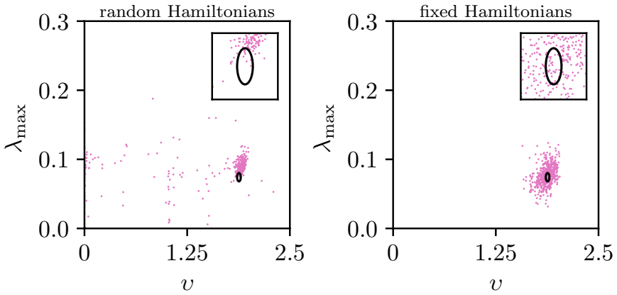
The load-bearing premise is that a random Hamiltonian draw from the specified ensemble gives a usable reservoir for every system, which the supplemental WINDMI experiment, where fixing one well-performing Hamiltonian raised the mean forecast horizon from 5.9 to 8.1 Lyapunov times and removed diverging trajectories, shows is not automatically true.

Editorial extensions

If this is right

Mean forecast horizons of roughly 12 Lyapunov times on five of eight benchmark systems put the four-qubit setup on par with, and in some cases ahead of, the classical and hybrid reservoir methods used for comparison in the paper.
For systems with good short-term skill, the same trained reservoir reproduces the attractor's largest Lyapunov exponent and correlation dimension within about five standard deviations across 500 realizations, meaning the model captures the underlying dynamics rather than merely memorizing the training segment.
Because the reservoir uses only four qubits, the approach sits within reach of current noisy intermediate-scale quantum hardware, and the supplemental dephasing experiments indicate forecast quality is maintained over a broad noise range.
The best hyperparameter configurations all use the maximal number of reservoirs considered, namely $r=3$, suggesting spatial multiplexing is load-bearing for small quantum reservoirs.
The three systems with shorter horizons, Chua, Thomas, and WINDMI, are also comparatively hard for conventional reservoir computing, so the failure pattern tracks the difficulty of the dynamical system rather than a quantum-specific defect.

Reading between the lines

Editorial extensions of the paper, not claims the author makes directly.

If the five-standard-deviation climate reproduction generalizes beyond the eight benchmarks, quantum reservoir computing could serve as a cheap generative model for chaotic attractors, producing synthetic trajectories with correct invariant measures for Monte Carlo or risk studies.
The supplemental WINDMI experiment suggests a practical protocol: draw several candidate Hamiltonians, score each on a short validation horizon, and freeze the best one, which could lift mean forecast horizons for hard systems without any structural change to the algorithm.
Because the encoding interval $[a,b]$ was explored only on a coarse grid, a continuous optimization of that interval might improve the three poorly predicted systems and could be tested with the same code.
A matched ablation against a classical echo-state network with a similar readout dimension and training budget would isolate what the four-qubit reservoir contributes, since the current comparison is against published classical baselines rather than identically tuned classical reservoirs.

Share X Bluesky LinkedIn Reddit HN

Editorial analysis

A structured set of objections, weighed in public.

Desk editor's note, referee report, and a circularity audit.

Desk Editor's Note

read the letter

Short version: this is a solid empirical benchmark with an overstated headline. What's actually new is the systematic statistical validation: eight 3D chaotic systems, 500 runs each, both short-term forecast horizons and long-term climate (Lyapunov exponent, correlation dimension) reproduced within about 5 sigma for five systems. The building blocks—temporal and spatial multiplexing, polynomial readout, ridge regression—are all published, but the combination and the scale of validation is new, and the claim that QRC can reproduce long-term climate is, as far as I know, new. The paper is honest about its weak spots: it flags the WINDMI behavior and discusses diverging trajectories and hyperparameter sensitivity.

The main problems are framing and statistical interpretation. First, every best configuration uses r=3 reservoirs, so the system is twelve qubits, not four. "Four-qubit systems" is literally true but the headline "minimal number of qubits necessary" is misleading. Second, the reported means and error bars are computed by averaging over 500 runs with a fresh random Hamiltonian draw each time. That mixes device-to-device variability with trajectory-to-trajectory variability. A physical reservoir has a fixed Hamiltonian; the user gets one draw. The paper's own Supplemental Note 3 shows this matters: fixing a well-performing Hamiltonian for WINDMI changes the mean forecast horizon from 5.9 ± 2.9 to 8.1 ± 2.6 Lyapunov times and eliminates the divergent climate trajectories. So the headline statistics describe an average over random devices, not the performance of any particular four-qubit device. The existence claim survives—there are good Hamiltonians—but the robustness claim is overstated.

Third, the hyperparameters are selected by maximizing the forecast horizon on the same metric, with no validation split, so the 500-run numbers are optimistic. And the classical baseline comes from a same-group paper, so the "rivaling classical RC" claim is not independently established. Code and data are "available upon request," which in practice means not available.

These are all addressable. I think the paper deserves a serious referee. The core demonstration—that a small quantum reservoir with classical polynomial readout can reproduce the climate of several chaotic systems—is interesting and, if confirmed with a fixed Hamiltonian and matched baseline, would be a useful result for the QRC community. My recommendation: send to peer review, but request a revision that (a) fixes the qubit accounting, (b) reports fixed-Hamiltonian results alongside the ensemble averages, and (c) releases code and data.

Referee Report

3 major / 6 minor

Summary. The paper proposes a quantum reservoir computing (QRC) pipeline for forecasting three-dimensional chaotic systems, combining four-qubit spin reservoirs with spatial and temporal multiplexing and polynomial readout functions. For eight benchmark systems, hyperparameters are selected by Bayesian optimization, and short-term (forecast horizon in Lyapunov times) and long-term (largest Lyapunov exponent and correlation dimension) performance are evaluated over 500 simulated runs. The authors report mean forecast horizons of about 3 to 13 Lyapunov times, accurate climate reproduction for five of the eight systems, and diverging trajectories for the remaining three. They conclude that QRC with very small qubit systems can rival classical reservoir computing and reproduce chaotic climate statistics.

Significance. The paper provides a useful empirical benchmark: eight chaotic systems, 500-run statistics, evaluation on unseen continuations, explicit hyperparameter optimization, and a noise supplement. If the results hold for a fixed small reservoir, they would support the promise of NISQ-era quantum reservoir computing and extend it to long-term climate reproduction. However, the headline claim of a "minimal" four-qubit reservoir is undermined by the fact that every best configuration uses three four-qubit reservoirs, and the main statistics average over random Hamiltonians rather than fixed devices. The paper's own WINDMI experiment shows that Hamiltonian choice substantially changes performance. These issues affect the central claim and need to be resolved before the results can be taken as stated.

major comments (3)

[Abstract; Sec. II.B; Table III (Supp. Note 2)] The central claim that the reservoir "consists of the minimal number of qubits necessary for this task, namely four" is not supported by the implemented architecture. The model uses r quantum systems, and Table III shows r = 3 for every best configuration, so the full reservoir comprises twelve qubits total (three independent four-qubit systems). If the claim is per-reservoir, the total resource count and the sense in which four is "minimal" must be stated explicitly; as written, the abstract and Sec. II.B conflate a four-qubit reservoir with a twelve-qubit multiplexed reservoir.
[Sec. II.B; Sec. IV.C; Supp. Note 3] The 500-run statistics in Table I and Fig. 1 are obtained by drawing a new random Hamiltonian from the ensemble of Eq. (15) for every run, while the text states "We choose a quantum system (unitary evolution) that works and do not further optimize it." A realized quantum reservoir has a fixed Hamiltonian, so the reported mean and standard deviation mix device-to-device variability with trajectory-to-trajectory variability and do not certify the performance of any fixed four-qubit device. Supp. Note 3 shows for WINDMI that fixing a well-performing Hamiltonian changes the mean forecast horizon from 5.9 +/- 2.9 to 8.1 +/- 2.6 Lyapunov times and removes strongly diverging climate trajectories; the authors should report fixed-Hamiltonian statistics for all systems, or demonstrate that the random-Hamiltonian average is representative of a typical fixed device.
[Sec. II.B] The claim that QRC "rival[s] and in some cases outperform[s] classical RC methods" is not verifiable from the manuscript: Table I contains only QRC results, and the comparison with Ref. [31] is described qualitatively with no table, figure, or numerical values for the classical or hybrid methods on the same systems and training sizes. Please provide a direct quantitative comparison, or explicitly restrict the claim to the comparisons actually shown.

minor comments (6)

[Eq. (13)] Equation (13) writes Wout = Y Q^T (Q Q^T - beta 1)^{-1}, but the ridge objective in Eq. (14) gives Wout = Y Q^T (Q Q^T + beta 1)^{-1}. The minus sign makes the matrix potentially singular or non-positive-definite; if the simulations used the plus sign, the equation should be corrected.
[Eq. (17)] The normalization in Eq. (17) uses a constant denominator <||y(t)||^2>^{1/2} averaged over all Npred steps, which makes e(t) a global rather than pointwise normalized error. Please define the normalization explicitly and state whether this choice affects the forecast-horizon threshold criterion.
[Abstract; Table I; Fig. 2] The abstract should qualify the long-term prediction claim: Table I and Fig. 2 show that Chua, Thomas, and WINDMI have mean forecast horizons of about 3 Lyapunov times, and WINDMI's predicted correlation dimension deviates by roughly 19 standard deviations from the true value. Only five of eight systems are accurately reproduced in climate.
[Data and Code Availability] Both the Data and Code Availability statements say "available from the corresponding author upon reasonable request." For a benchmark paper whose claims rest on 500-run simulations, I recommend depositing the code and data in a permanent repository to allow independent reproduction.
[Eq. (2)] The notation in Eq. (2) has an extra closing parenthesis and should clarify that after the partial trace over the first d qubits, the new input state is encoded into those qubits; as written the state rho_k is not fully defined.
[Sec. III] There is a typo in Sec. III: "learn patters" should read "learn patterns." Also, the title and abstract should use "four-qubit systems" or "four qubits per reservoir" consistently to avoid ambiguity.

Circularity Check

0 steps flagged · score 0.0 of 10

No significant circularity: the QRC benchmark is self-contained; the readout is trained on one-step-ahead targets and the reported metrics are evaluated on unseen continuations.

full rationale

The derivation chain is not circular. The reservoir output q(k) is constructed from the encoding, unitary evolution, and readout functions in Eqs. (2)-(9); the only fitted quantity is the readout matrix Wout, obtained by ridge regression in Eq. (13) against the one-step-ahead training targets Y, not against the forecast horizon or climate measures. Prediction is closed-loop use of Eq. (12) on continuations that were not used in training, and the forecast horizon and climate statistics are computed from those continuations. Hyperparameter selection by Bayesian optimization of mean forecast horizon over Nstat=100 runs is standard model selection; the reported Nstat=500 statistics use new attractor segments and new Hamiltonian draws, so the reported values are not forced equal to the optimization objective by construction. The Hamiltonian parameters in Sec. IV C are adopted from the independent prior work of Martinez-Pena et al. (Ref. [16]), not from the present authors; the nonlinear readout scheme is defined explicitly in the paper and its citation to Ref. [29] is a published, externally checkable technique rather than a load-bearing self-citation. The comparisons to Ref. [31] and the evaluation measures from Refs. [33-35] are published benchmarks and do not reduce the present results to the authors' own definitions. Supplement Note 3 explicitly shows that fixing a well-performing Hamiltonian changes WINDMI's mean forecast horizon from 5.9 to 8.1 Lyapunov times, and Supplement Note 5 states the simulations are noiseless; these are robustness and applicability limitations, not circular steps, because the main-text statistics average over random Hamiltonians and the fixed-Hamiltonian experiment is a separate diagnostic. No equation in the paper defines a prediction target in terms of the fitted readout or defines the reservoir in terms of the predicted quantities, so no circularity is present.

Assumptions & free parameters 6 free parameters · 5 assumptions · 0 invented entities

The paper introduces no new physical entities. Its central claim rests on five domain assumptions about the quantum reservoir, plus per-system fitted hyperparameters listed in Supplemental Table III. The free parameter count is significant: six hyperparameters (V, r, beta, G, [a, b], and in the WINDMI supplement the Hamiltonian realization) are tuned to maximize the reported forecast horizon.

free parameters (6)

V (number of evolution and measurement cycles per input step) = 9, 8, 14, 8, 9, 7, 15, 10 for Lorenz-63, Chen, Chua, Halvorsen, Rössler, Rucklidge, Thomas, WINDMI (Supplemental Table…
Optimized per system by Optuna Bayesian search to maximize mean forecast horizon (Sec. II.B).
r (number of spatial multiplexing reservoirs) = 3 for all systems
Optimized over {1, 2, 3}; every best configuration uses the maximum, so the total qubit count is 3 x 4 = 12.
beta (ridge regression parameter) = from 1.09e-12 to 0.000269 depending on system (Supplemental Table III)
Optimized per system; Supplemental Note 1 shows that extreme beta values cause diverging or periodic predictions.
G (polynomial readout degree) = 2 for Chua, 3 for Lorenz, Chen, Halvorsen, Rössler, 4 for Rucklidge, Thomas, WINDMI
Optimized per system; higher degrees increase the dimension of the readout vector.
Encoding interval [a, b] = various, e.g. [0.15, 0.85], [0.10, 0.90], [0.05, 0.95] (Supplemental Table III)
Selected from a discrete set and optimized per system; Sec. III calls the investigation of a and b "very simplistic."
Random Hamiltonian couplings Jij and disorders Di = not fitted in the main text; one well-performing realization selected for WINDMI in Supplemental Note 3
Random draws from uniform intervals in Eq. (15). Supplemental Note 3 shows that choosing a good draw changes the WINDMI mean forecast horizon from 5.9 to 8.1 Lyapunov times, so the realization is effectively a performance-relevant stochastic parameter.

assumptions (5)

domain assumption The four-qubit reservoir states maintain a fading memory of the input history (echo state property) for the chosen encoding and Hamiltonian.
The readout in Eq. (11) relies on the reservoir response encoding current and past inputs (Secs. II.A and IV.A); no proof or memory-capacity analysis is given.
domain assumption The fixed Hamiltonian parameter set tau = 20J, h = 2/J, W = 0.05/J, J = 1 from Ref. [16] defines a working reservoir for all eight systems without further optimization.
Sec. IV.C states "We choose a quantum system (unitary evolution) that works and do not further optimize it"; the WINDMI supplement shows this assumption does not hold equally for all random realizations.
domain assumption The observables <sigma_z^i> and <sigma_z^i sigma_z^l>, together with elementwise powers up to degree G <= 4, provide a sufficient readout.
Sec. IV.A defines the output nodes; no completeness or information-theoretic argument is given.
domain assumption Standardization followed by scaling into the interval [a, b] preserves the dynamics needed for prediction.
Sec. II.A introduces a and b as preprocessing hyperparameters; Supplemental Note 1 shows the optimal choice depends on the other hyperparameters.
standard math The Rosenstein and Grassberger-Procaccia algorithms give unbiased estimates of the largest Lyapunov exponent and correlation dimension for both true and predicted 20000-step trajectories.
Sec. IV.D uses these standard estimators; the predicted WINDMI correlation dimension (1.88 vs true 1.5, with a much narrower spread) suggests estimator reliability can differ on forecasted data.

how reviews work

0 comments

Cite this review

Pith. "Pith review of Predicting three-dimensional chaotic systems with four qubit quantum systems." pith.science (2026). https://pith.science/paper/3EFU3AW4

@misc{pith2026250115191,
  author       = {Pith},
  title        = {Pith review of: Predicting three-dimensional chaotic systems with four qubit quantum systems},
  year         = {2026},
  howpublished = {\url{https://pith.science/paper/3EFU3AW4}},
  note         = {Machine review of arXiv:2501.15191}
}

read the original abstract

Reservoir computing (RC) is among the most promising approaches for AI-based prediction models of complex systems. It combines superior prediction performance with very low CPU-needs for training. Recent results demonstrated that quantum systems are also well-suited as reservoirs in RC. Due to the exponential growth of the Hilbert space dimension obtained by increasing the number of quantum elements small quantum systems are already sufficient for time series prediction. Here, we demonstrate that three-dimensional systems can already well be predicted by quantum reservoir computing with a quantum reservoir consisting of the minimal number of qubits necessary for this task, namely four. This is achieved by optimizing the encoding of the data, using spatial and temporal multiplexing and recently developed read-out-schemes that also involve higher exponents of the reservoir response. We outline, test and validate our approach using eight prototypical three-dimensional chaotic systems. Both, the short-term prediction and the reproduction of the long-term system behavior (the system's "climate") are feasible with the same setup of optimized hyperparameters. Our results may be a further step towards the realization of a dedicated small quantum computer for prediction tasks in the NISQ-era.

Figures

Figures reproduced from arXiv: 2501.15191 by the authors.

**Figure 1.** FIG. 1. Distributions of the short-term accuracy for all eight forecasted chaotic systems. These are shown in a boxplot of the [PITH_FULL_IMAGE:figures/full_fig_p004_1.png] view at source ↗

**Figure 2.** FIG. 2. Distributions of the predicted climate for all eight forecasted chaotic systems. These are depicted by showing the [PITH_FULL_IMAGE:figures/full_fig_p005_2.png] view at source ↗

**Figure 3.** FIG. 3. Schematic illustration of the prediction phase of the [PITH_FULL_IMAGE:figures/full_fig_p006_3.png] view at source ↗

Figures from the paper (14 more)

**Figure 11.** Figure 11: The right choice of [a,b] seems to critically depend on the other hyperparameters. configuration label V r G [a, b] dim(q(k)) configuration 1 3 1 1 [0.10, 0.90] 31 configuration 2 4 2 3 [0.20, 0.80] 241 configuration 3 5 1 1 [0.20, 0.80] 51 configuration 4 5 1 2 [0.15…

**Figure 1.** Figure 1: FIG. 1. Example of a trajectory of one of the 500 continued time series (TABLE III) obtained [PITH_FULL_IMAGE:figures/full_fig_p012_1.png]

**Figure 2.** Figure 2: FIG. 2. Example of a trajectory of the predic [PITH_FULL_IMAGE:figures/full_fig_p012_2.png]

**Figure 4.** Figure 4: FIG. 4. Boxplot of the forecast horizon in Lyapunov times of 100 forecasted trajectories of the [PITH_FULL_IMAGE:figures/full_fig_p013_4.png]

**Figure 5.** Figure 5: FIG. 5. Boxplot (100 forecasted trajectories) presenting the forecast horizon of the prediction of [PITH_FULL_IMAGE:figures/full_fig_p014_5.png]

**Figure 6.** Figure 6: FIG. 6. Boxplot (100 forecasted trajectories) presenting the forecast horizon of the prediction of [PITH_FULL_IMAGE:figures/full_fig_p014_6.png]

**Figure 7.** Figure 7: FIG. 7. Boxplot (100 forecasted trajectories) presenting the forecast horizon of the prediction of [PITH_FULL_IMAGE:figures/full_fig_p014_7.png]

**Figure 8.** Figure 8: FIG. 8. Scatter plots of the predicted forecast horizons showing the predicted [PITH_FULL_IMAGE:figures/full_fig_p015_8.png]

**Figure 9.** Figure 9: FIG. 9. Largest Lyapunov exponent scattered against correlation dimension 100 forecasted trajec [PITH_FULL_IMAGE:figures/full_fig_p016_9.png]

**Figure 10.** Figure 10: FIG. 10. Largest Lyapunov exponent scattered against correlation dimension 100 forecasted tra [PITH_FULL_IMAGE:figures/full_fig_p017_10.png]

**Figure 11.** Figure 11: FIG. 11. Largest Lyapunov exponent scattered against correlation dimension 100 forecasted [PITH_FULL_IMAGE:figures/full_fig_p018_11.png]

**Figure 12.** Figure 12: FIG. 12. Predicted climate for each of the 500 forecasted trajectories of the WINDMI system as [PITH_FULL_IMAGE:figures/full_fig_p021_12.png]

**Figure 13.** Figure 13: FIG. 13. Forecast horizon for randomly drawn Hamiltonians and fixed (well performing) Hamilto [PITH_FULL_IMAGE:figures/full_fig_p021_13.png]

**Figure 14.** Figure 14: FIG. 14. Forecast horizon of the prediction of the Lorenz system obtained by noisy quantum [PITH_FULL_IMAGE:figures/full_fig_p024_14.png]

Discussion (0). Continue with ORCID to comment.

Reference graph

Works this paper leans on

52 extracted references · 37 canonical work pages

[31]

Duncan and C

D. Duncan and C. R¨ ath, Optimizing the combi- nation of data-driven and model-based elements in hybrid reservoir computing, Chaos: An In- terdisciplinary Journal of Nonlinear Science 33, 103109 (2023), https://pubs.aip.org/aip/cha/article- pdf/doi/10.1063/5.0164013/18159235/103109 1 5.0164013.pdf

work page doi:10.1063/5.0164013/18159235/103109 2023
[1]

S. L. Brunton and J. N. Kutz, Data-Driven Science and Engineering: Machine Learning, Dynamical Sys- tems, and Control (Cambridge University Press, 2019)

work page 2019
[2]

Y. Tang, J. Kurths, W. Lin, E. Ott, and L. Kocarev, In- troduction to Focus Issue: When machine learning meets complex systems: Networks, chaos, and nonlinear dy- namics, Chaos: An Interdisciplinary Journal of Nonlinear Science 30, 063151 (2020)

work page 2020
[3]

The continued time series is denoted as ypred(t) = {ok}L+Npred k=L+1 in the following. B. Ridge Regression Ridge regression is used to obtain the readout matrix Wout by calculating Wout = YQT(QQT−β1)−1 (13) step k+1 1 1 V V step k+1 U U U U Fres ρ1 ρr ρr ρr ρ1 ρ1 q(k) Wout o1k o2k odk step k+1 U U FIG. 3. Schematic illustration of the prediction phase of ...

work page
[4]

Maass, T

W. Maass, T. Natschl¨ ager, and H. Markram, Real-time computing without stable states: A new framework for neural computation based on perturbations, Neural Com- putation 14, 2531 (2002)

2002
[5]

Prokhorov, Echo state networks: appeal and chal- lenges, in Proceedings

D. Prokhorov, Echo state networks: appeal and chal- lenges, in Proceedings. 2005 IEEE International Joint Conference on Neural Networks, 2005. , Vol. 3 (2005) pp. 1463–1466

work page 2005
[6]

Jaeger, The”echo state”approach to analysing and training recurrent neural networks (2001)

H. Jaeger, The”echo state”approach to analysing and training recurrent neural networks (2001)

work page 2001
[7]

Pathak, Z

J. Pathak, Z. Lu, B. Hunt, M. Girvan, and E. Ott, Us- ing machine learning to replicate chaotic attractors and calculate lyapunov exponents from data, Chaos: An In- terdisciplinary Journal of Nonlinear Science 27 (2017)

work page 2017

Show all 52 references

[8]

Pathak, B

J. Pathak, B. Hunt, M. Girvan, Z. Lu, and E. Ott, Model- free prediction of large spatiotemporally chaotic systems from data: A reservoir computing approach, Phys. Rev. Lett. 120, 024102 (2018)

2018
[9]

Z. Lu, J. Pathak, B. Hunt, M. Girvan, R. Brockett, and E. Ott, Reservoir observers: Model-free inference of un- measured variables in chaotic systems, Chaos: An In- terdisciplinary Journal of Nonlinear Science 27, 041102 (2017)

2017
[10]

R. S. Zimmermann and U. Parlitz, Observing spatio- temporal dynamics of excitable media using reservoir computing, Chaos: An Interdisciplinary Journal of Non- linear Science 28, 043118 (2018)

2018
[11]

L.-W. Kong, G. Brewer, and Y.-C. Lai, Reservoir- computing based associative memory and itinerancy for complex dynamical attractors, Nature Communications 15 (2024)

2024
[12]

Z. Lu, B. R. Hunt, and E. Ott, Attractor reconstruction by machine learning, Chaos: An Interdisciplinary Jour- nal of Nonlinear Science 28, 061104 (2018)

2018
[14]

Fujii and K

K. Fujii and K. Nakajima, Quantum reservoir computing: a reservoir approach toward quantum machine learning on near-term quantum devices (2020), arXiv:2011.04890 [quant-ph]

2020 arXiv
[15]

X. Li, Q. Zhu, C. Zhao, X. Duan, B. Zhao, X. Zhang, H.- F. Ma, J. Sun, and W. Lin, Higher-order granger reservoir computing: Simultaneously achieving scalable complex structures inference and accurate dynamics prediction, Nature Communications 15, 2506 (2024)

2024
[16]

Mart´ ınez-Pe˜ na, G

R. Mart´ ınez-Pe˜ na, G. L. Giorgi, J. Nokkala, M. C. So- riano, and R. Zambrini, Dynamical phase transitions in quantum reservoir computing, Phys. Rev. Lett. 127, 100502 (2021)

2021
[17]

Chen and H

J. Chen and H. I. Nurdin, Learning nonlinear in- put–output maps with dissipative quantum systems, Quantum Information Processing 18, 10.1007/s11128- 019-2311-9 (2019)

2019 doi
[18]

Nakajima, K

K. Nakajima, K. Fujii, M. Negoro, K. Mitarai, and M. Kitagawa, Boosting computational power through spatial multiplexing in quantum reservoir comput- ing, Physical Review Applied 11, 10.1103/physrevap- plied.11.034021 (2019)

2019 doi
[19]

Q. H. Tran and K. Nakajima, Higher-order quantum reservoir computing (2020), arXiv:2006.08999 [quant-ph]

2020 arXiv
[20]

unitary operator choices are investigated that might be more suitable for applications in the near-term fu- ture. The model introduced in our work is applicable to other unitary operators and therefore gives a good start- ing point for further research towards employing small ...
[21]

Mart´ ınez-Pe˜ na, J

R. Mart´ ınez-Pe˜ na, J. Nokkala, G. L. Giorgi, R. Zambrini, and M. C. Soriano, Information processing capacity of spin-based quantum reservoir computing systems, Cog- nitive Computation 15, 1440–1451 (2020)

2020
[22]

Ghosh, T

S. Ghosh, T. Paterek, and T. C. H. Liew, Quantum neuromorphic platform for quantum state preparation., Physical review letters 123 26 , 260404 (2019)

2019
[23]

Domingo, M

L. Domingo, M. Grande, G. Carlo, F. Borondo, and J. Borondo, Optimal quantum reservoir computing for market forecasting: An application to fight food price crises, (2023), arXiv:2401.03347 [quant-ph]

2023 arXiv
[24]

Ghosh, A

S. Ghosh, A. Opala, M. Matuszewski, T. Paterek, and T. C. H. Liew, Quantum reservoir processing, npj Quan- tum Information 5, 10.1038/s41534-019-0149-8 (2019)

2019 doi
[25]

Mujal, R

P. Mujal, R. Mart´ ınez-Pe˜ na, J. Nokkala, J. Garc´ ıa-Beni, G. L. Giorgi, M. C. Soriano, and R. Zambrini, Opportu- nities in quantum reservoir computing and extreme learn- ing machines, Advanced Quantum Technologies4 (2021)

2021
[26]

J. Chen, H. I. Nurdin, and N. Yamamoto, Temporal infor- mation processing on noisy quantum computers, Physical Review Applied 14, 10.1103/physrevapplied.14.024065 (2020)

2020 doi
[27]

Negoro, K

M. Negoro, K. Mitarai, K. Fujii, K. Nakajima, and M. Kitagawa, Machine learning with controllable quan- tum dynamics of a nuclear spin ensemble in a solid (2018), arXiv:1806.10910 [quant-ph]. 9

2018 arXiv
[28]

J. Lau, K. Lim, H. Shrotriya, and L. Kwek, Nisq comput- ing: where are we and where do we go?, AAPPS Bulletin 32 (2022)

2022
[29]

Preskill, Quantum Computing in the NISQ era and beyond, Quantum 2, 79 (2018)

J. Preskill, Quantum Computing in the NISQ era and beyond, Quantum 2, 79 (2018)

2018
[30]

Bharti, A

K. Bharti, A. Cervera-Lierta, T. H. Kyaw, T. Haug, S. Alperin-Lea, A. Anand, M. Degroote, H. Heimonen, J. S. Kottmann, T. Menke, W.-K. Mok, S. Sim, L.-C. Kwek, and A. Aspuru-Guzik, Noisy intermediate-scale quantum algorithms, Reviews of Modern Physics 94, 10.1103/revmodphys.94...

2022 doi
[32]

H. Ma, D. Prosperino, and C. R¨ ath, A novel approach to minimal reservoir computing, Scientific Reports 13 (2023)

2023
[33]

Akiba, S

T. Akiba, S. Sano, T. Yanase, T. Ohta, and M. Koyama, Optuna: A next-generation hyperparameter optimiza- tion framework (2019), arXiv:1907.10902 [cs.LG]

2019 arXiv
[34]

Haluszczynski, J

A. Haluszczynski, J. Aumeier, J. Herteux, and C. R¨ ath, Reducing network size and improving prediction stability of reservoir computing, Chaos: An In- terdisciplinary Journal of Nonlinear Science 30, 063136 (2020), https://pubs.aip.org/aip/cha/article- pdf/doi/10.1063/5.00068...

2020 doi
[35]

Giammarese, K

A. Giammarese, K. Rana, E. M. Bollt, and N. Malik, Tree-based learning for high-fidelity prediction of chaos (2024), arXiv:2403.13836 [cs.LG]

2024 arXiv
[36]

Haluszczynski and C

A. Haluszczynski and C. R¨ ath, Good and bad predic- tions: Assessing and improving the replication of chaotic attractors by means of reservoir computing, Chaos: An Interdisciplinary Journal of Nonlinear Science 29, 103143 (2019), https://pubs.aip.org/aip/cha/article- pdf/doi/...

2019 doi
[37]

Grassberger and I

P. Grassberger and I. Procaccia, Measuring the strangeness of strange attractors, Physica D: Nonlinear Phenomena 9, 189 (1983)

1983
[38]

Another characteristic of the long-term climate of a sys- tem is its temporal complexity

is used to calculate the correlation dimension from data. Another characteristic of the long-term climate of a sys- tem is its temporal complexity. The most appropriate way to quantify the temporal complexity of a dynamical system is to analyze its Lyapunov exponents, characte...
[39]

Herteux and C

J. Herteux and C. R¨ ath, Breaking symmetries of the reservoir equations in echo state networks, Chaos: An Interdisciplinary Journal of Nonlinear Science 30, 123142 (2020), https://pubs.aip.org/aip/cha/article- pdf/doi/10.1063/5.0028993/14110522/123142 1 online.pdf

2020 doi
[40]

Pathak, A

J. Pathak, A. Wikner, R. Fussell, S. Chandra, B. R. Hunt, M. Girvan, and E. Ott, Hybrid forecasting of chaotic processes: Using machine learning in con- junction with a knowledge-based model, Chaos: An Interdisciplinary Journal of Nonlinear Science 28, 041101 (2018), https://p...

2018 doi
[41]

Grassberger, Generalized dimensions of strange attrac- tors, Physics Letters A 97, 227 (1983)

P. Grassberger, Generalized dimensions of strange attrac- tors, Physics Letters A 97, 227 (1983)

1983
[42]

A. Wolf, J. Swift, H. L. Swinney, and J. A. Vastano, De- termining lyapunov exponents from a time series, Physica D: Nonlinear Phenomena 16, 285 (1985)

1985
[43]

Shaw, Strange attractors, chaotic behavior, and in- formation flow, Zeitschrift f¨ ur Naturforschung A36, 80 (1981)

R. Shaw, Strange attractors, chaotic behavior, and in- formation flow, Zeitschrift f¨ ur Naturforschung A36, 80 (1981)

1981
[44]

M. T. Rosenstein, J. J. Collins, and C. J. De Luca, A practical method for calculating largest lyapunov expo- nents from small data sets, Physica D: Nonlinear Phe- nomena 65, 117 (1993). Supplemental information Predicting three-dimensional chaotic systems with four qubit quan...

1993
[45]

A very large regression parameter ( β = 10) typically leads to periodic predictions like in Fig. 3. These extreme parameter choices result in models that we can characterize as not working. This illustrates that the regression parameter has to be carefully optimized to 1 arXiv...

2025 arXiv
[46]

11 0 1.25 2.5 υ 0.0 0.1 0.2 0.3 λmax ﬁxed Hamiltonians 0 1.25 2.5 υ 0.0 0.1 0.2 0.3 λmax random Hamiltonians FIG

It is clear that using a ”well-performing” combination of unitary operators leads to the disappearance of the predicted trajectories that deviate after very short time scales from the real continuation of the time series, and also results in accurate climate prediction. 11 0 1...

2000
[47]

As the noise increases further, the forecast horizon shortens, but the prediction does not completely break down

One can observe that for a large range of γ, the prediction remains accurate on longer timescales compared to the noiseless case (γ = 0). As the noise increases further, the forecast horizon shortens, but the prediction does not completely break down. 0 10 −10 10−9 10−8 10−7 1...
[48]

Fujii and K

K. Fujii and K. Nakajima, Harnessing disordered-ensemble quantum dynamics for machine learning, Physical Review Applied 8, 10.1103/physrevapplied.8.024030 (2017)

2017 doi
[49]

Runge, Ueber die numerische aufl¨ osung von differentialgleichungen., Mathematische Annalen 46, 167 (1895)

C. Runge, Ueber die numerische aufl¨ osung von differentialgleichungen., Mathematische Annalen 46, 167 (1895)
[50]

Kutta, Beitrag zur n¨ aherungsweisen Integration totaler Differentialgleichungen, Zeit

W. Kutta, Beitrag zur n¨ aherungsweisen Integration totaler Differentialgleichungen, Zeit. Math. Phys. 46, 435 (1901)

1901
[51]

Sprott, Chaos and Time-series Analysis (Oxford University Press, 2003)

J. Sprott, Chaos and Time-series Analysis (Oxford University Press, 2003)

2003
[52]

Domingo, G

L. Domingo, G. Carlo, and F. Borondo, Taking advantage of noise in quantum reservoir com- puting, Scientific Reports 13, 10.1038/s41598-023-35461-5 (2023)

2023 doi
[53]

Johansson, P

J. Johansson, P. Nation, and F. Nori, Qutip 2: A python framework for the dynamics of open quantum systems, Computer Physics Communications 184, 1234 (2013). 16

2013

Pith tools

Reviewed August 10, 2026 · model on record in the stance chip above.

[1] [31]

Duncan and C

D. Duncan and C. R¨ ath, Optimizing the combi- nation of data-driven and model-based elements in hybrid reservoir computing, Chaos: An In- terdisciplinary Journal of Nonlinear Science 33, 103109 (2023), https://pubs.aip.org/aip/cha/article- pdf/doi/10.1063/5.0164013/18159235/103109 1 5.0164013.pdf

work page doi:10.1063/5.0164013/18159235/103109 2023

[2] [1]

S. L. Brunton and J. N. Kutz, Data-Driven Science and Engineering: Machine Learning, Dynamical Sys- tems, and Control (Cambridge University Press, 2019)

work page 2019

[3] [2]

Y. Tang, J. Kurths, W. Lin, E. Ott, and L. Kocarev, In- troduction to Focus Issue: When machine learning meets complex systems: Networks, chaos, and nonlinear dy- namics, Chaos: An Interdisciplinary Journal of Nonlinear Science 30, 063151 (2020)

work page 2020

[4] [3]

The continued time series is denoted as ypred(t) = {ok}L+Npred k=L+1 in the following. B. Ridge Regression Ridge regression is used to obtain the readout matrix Wout by calculating Wout = YQT(QQT−β1)−1 (13) step k+1 1 1 V V step k+1 U U U U Fres ρ1 ρr ρr ρr ρ1 ρ1 q(k) Wout o1k o2k odk step k+1 U U FIG. 3. Schematic illustration of the prediction phase of ...

work page

[5] [4]

Maass, T

W. Maass, T. Natschl¨ ager, and H. Markram, Real-time computing without stable states: A new framework for neural computation based on perturbations, Neural Com- putation 14, 2531 (2002)

2002

[6] [5]

Prokhorov, Echo state networks: appeal and chal- lenges, in Proceedings

D. Prokhorov, Echo state networks: appeal and chal- lenges, in Proceedings. 2005 IEEE International Joint Conference on Neural Networks, 2005. , Vol. 3 (2005) pp. 1463–1466

work page 2005

[7] [6]

Jaeger, The”echo state”approach to analysing and training recurrent neural networks (2001)

H. Jaeger, The”echo state”approach to analysing and training recurrent neural networks (2001)

work page 2001

[8] [7]

Pathak, Z

J. Pathak, Z. Lu, B. Hunt, M. Girvan, and E. Ott, Us- ing machine learning to replicate chaotic attractors and calculate lyapunov exponents from data, Chaos: An In- terdisciplinary Journal of Nonlinear Science 27 (2017)

work page 2017