REVIEW 4 major objections 4 minor 43 references
CIBER 4th flight fluctuation analysis: Pseudo-power spectrum formalism, improved source masking and validation on mocks
T0 review · 4 major / 4 minor · reviewed 2026-08-10 · deepseek-v4-flash
Pith's one-line read This paper shows that CIBER can recover unbiased near-infrared sky fluctuation power spectra from single fields by correcting flat-field errors in the pseudo-power-spectrum domain and by masking point sources two magnitudes deeper than…
desk verdict Careful FF-corrected pseudo-C_l formalism and a useful masking technique, but the abstract's <10% shot-noise claim contradicts Table 2 and the unbiased-recovery validation skips masking errors. read the letter →
The pith
A machine-rendered reading of the paper's core claim, the machinery that carries it, and where it could break.
The reading
What carries the argument
The load-bearing object is the extended pseudo-$C_\ell$ mode-mixing matrix $M_{\ell\ell'}$, which in this paper combines the survey mask, the flat-field stacking estimator, and the image filter into one linear operation. Additive flat-field noise bias is subtracted through modified Monte Carlo noise realizations that include mean sky levels and flat-field stacking; the multiplicative flat-field bias, which scales with the ratio of mean sky brightnesses between target and off-fields, is corrected analytically in the unmasked limit and included in the matrix for the masked case. The source-masking component is a random forest regressor trained on UKIDSS UDS photometry that maps PanSTARRS and unWISE magnitudes to predicted J and H magnitudes, with mask radii set by iteratively suppressing extended PSF power.
What would settle it
Run the pipeline on mocks in which the off-field sky fluctuations are drawn from a different power spectrum than the target field, such as one field with suppressed large-scale diffuse galactic light, and check whether the recovered target power spectrum remains unbiased after the multiplicative correction; alternatively, inject the masking errors quantified in Section 6, such as 0.25-pixel astrometric scatter or the ten-to-twenty percent completeness gaps, directly into the mock validation and see whether the claimed unbiased recovery on scales $500<\ell<2000$ survives.
Extended reading notes
Core claim
The central claim is that flat-field errors, which previously forced CIBER to analyze differences between fields, can instead be corrected directly in the pseudo-power-spectrum domain. The flat field is estimated by stacking per-field sky flats from the four other science fields, and the resulting errors are propagated into two biases: an additive noise bias from instrument noise and a multiplicative bias of order $1+\sum_i (w_i I_j/I_i)^2$ from sky fluctuations. Both are folded into a mode-mixing matrix that is estimated with Monte Carlo tone realizations, so masked, filtered, flat-field-corrected maps recover the input sky power spectrum after inversion. The paper further claims that random forest regression on PanSTARRS and unWISE photometry predicts J- and H-band magnitudes with more than ninety percent completeness and purity relative to UKIDSS UDS validation, allowing masks two magnitudes deeper than 2MASS completeness while keeping fractional shot-noise errors below ten percent. Mock tests with injected laboratory flat fields demonstrate unbiased recovery for all but the smallest angular scales and quantify the residual flat-field penalty as less than twenty percent on $500<\ell<2000$.
Load-bearing premise
The multiplicative flat-field correction assumes that the sky fluctuations in the off-fields are drawn from the same underlying power spectrum as the target field and that foreground point sources are removed perfectly, so any field-to-field difference in the foreground spectrum or any masking error enters the final power spectrum uncorrected.
Editorial extensions
If this is right
- Single-field power spectra become usable, so the effective mask is no longer the union of two field masks and masking can be more aggressive.
- Residual flat-field error contributes less than twenty percent to the power-spectrum uncertainty on arcminute scales, so the fourth-flight dataset gains sensitivity without field differencing.
- Masking two magnitudes deeper reduces Poisson shot noise from unmasked sources while keeping shot-noise errors below ten percent at all tested depths.
- The pipeline yields field-averaged power spectra and covariances from mock ensembles that can be used to test field-to-field consistency in the real data.
- The formalism extends directly to cross-power spectra, with an analogous multiplicative flat-field bias correction, and to future instruments with similar imaging characteristics.
Reading between the lines
- A natural next test is to inject realistic masking errors, such as position noise, magnitude scatter, and catalog incompleteness, into the mocks; the current validation assumes perfect mask knowledge, so the unbiased-recovery claim has not yet been stress-tested against the masking systematics the paper itself characterizes.
- The multiplicative-bias formula suggests that in surveys with large field-to-field sky-brightness variation, the flat-field stacking estimator could be redesigned to down-weight bright fields, reducing the bias rather than correcting it after the fact.
- The random forest magnitude predictions could be turned into a de-projection method that subtracts rather than masks bright sources, which would preserve more Fourier modes on small scales.
- For future wide-area surveys, the common-spectrum assumption underlying the flat-field correction will likely need to be replaced by a forward model that marginalizes over variations in diffuse galactic light and integrated stellar light across fields.
Editorial analysis
A structured set of objections, weighed in public.
Referee Report
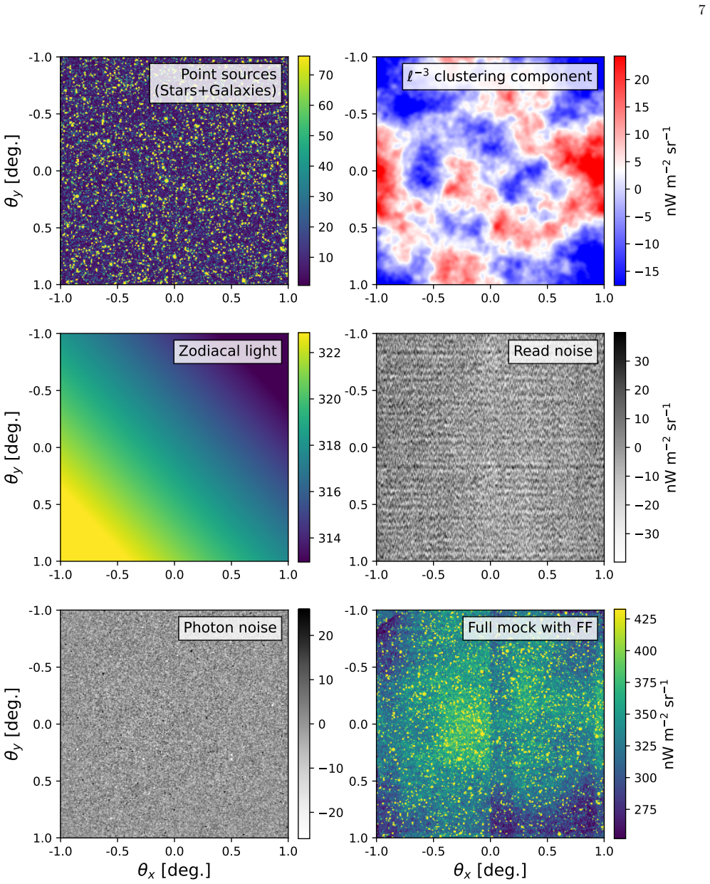
Summary. This methodology paper presents the analysis framework for the fourth CIBER flight, with two main innovations: a pseudo-power-spectrum formalism that corrects for additive and multiplicative biases from an in-flight flat-field (FF) stacking estimator, and a random-forest-based source masking method that uses PanSTARRS and unWISE photometry to predict J- and H-band magnitudes, allowing deeper masking than 2MASS alone. The authors validate the pipeline on 1000 synthetic CIBER observations that include realistic sky signals, noise, masks, filtering, and injected lab-derived FFs. They report unbiased recovery of sky fluctuations except on the smallest angular scales, with residual FF errors increasing uncertainties by less than 20% on scales 500 < ell < 2000, and shot-noise errors below 10% at all masking depths considered. The paper is written as a methods paper preceding a companion analysis of CIBER data.
Significance. If the claims hold, this is a valuable methodological contribution for CIBER and for future NIR intensity-mapping experiments such as CIBER-2 and SPHEREx. The derivation in Appendix A is careful and the use of a large mock ensemble to quantify biases, covariances, and field weights is a clear strength. The random-forest masking approach is well motivated and includes an out-of-sample test on COSMOS, which is a useful check of distribution shift. The paper also correctly identifies and quantifies several non-trivial effects, such as the coupling of FF errors with masks and the need to include filtering in the mode-mixing matrix. However, the central 'unbiased recovery' claim is currently stated more strongly than the evidence supports, because the mock tests assume perfect masking and because several known residual biases are acknowledged in the text. The tension between the abstract's <10% shot-noise claim and the deeper-mask entries in Table 2 also needs to be resolved before the paper is ready for publication.
major comments (4)
- [Abstract and Section 6.3, Table 2] The abstract states that shot-noise errors remain below <10% 'at all masking depths considered,' but Table 2 reports fractional shot-noise biases of -21.7% for J<19.0 and -16.4% for H<18.5, and the text in Section 6.3 acknowledges 22% and 16% departures at the deepest cuts. These deepest cuts are precisely where the claimed two-magnitude improvement over 2MASS is demonstrated, so the <10% claim is not supported as written. Please either correct the abstract and Section 6.3 to state the depth-dependent range and explicitly report the deepest-cut values, or revise the masking method so that the shot-noise errors are below 10% at all depths claimed.
- [Section 7] The mock recovery tests explicitly assume perfect knowledge of source masking: 'we assume perfect knowledge for source masking, i.e., we do not directly emulate masking errors.' The central conclusion that the pipeline 'can recover unbiased power spectra' is therefore conditional on perfect masks. The source-masking method is validated separately at catalog level in Section 6.3, but the fractional shot-noise biases measured there are never propagated through the FF-corrected pseudo-C_ell pipeline. Since the FF stacking estimator depends on the masks (Section 5.2.2) and Section 7.5 states that bright unmasked point sources break the matrix formalism, mask incompleteness or impurity could couple into FF errors and bias C_ell on exactly the scales where the paper claims <20% FF-induced uncertainty growth (500 < ell < 2000). The validation would be complete if masking errors were injected into the mock pipeline using the measured completeness and purity of the predicted catalogs, or if a quantitative propagation of the Section 6.3 shot-noise errors to recovered C_ell were provided.
- [Section 7.2 and Section 8] The paper claims unbiased recovery 'for all but the smallest angular scales,' yet Section 7.2 reports a negative bias at the fifth bandpower at the 1-2 sigma level in both the delta[FF]=0 and delta[FF]!=0 cases, and a positive bias at ell>50000 in the delta[FF]!=0 case. The fifth bandpower is not one of the smallest angular scales, so the Section 8 claim is not supported as stated. Please quantify these biases (amplitude relative to statistical error, field dependence, and whether they persist with more realizations) and either adjust the conclusions to list these exceptions or reduce the biases with additional corrections.
- [Section 7.5] The varying-masking-depth analysis relies on an empirical switch between M^{mask+filter} and M^{mask+filter+FF} at (Jlim,Hlim)=15 because the matrix formalism breaks down with bright unmasked point sources. This is a reasonable pragmatic choice, but it means the FF bias correction is not exact for shallow cuts, and the text notes a slight underestimation at (Jlim,Hlim)=16. The robustness of the large-angle science results to this approximation should be stated explicitly in the conclusions, since the companion paper will use these masks and readers may otherwise infer that the full pipeline is uniformly validated across all masking depths.
minor comments (4)
- [Section 7.2] There is a typo in the sentence describing the third-bandpower bias: 'however this is not seen in the The bias is not delta[FF] != 0 case' should be 'however this is not seen in the delta[FF] != 0 case.'
- [Section 7.5] The sentence 'In practice we use the J < 17.5 and H < 17.0 masks to calculate FFhat for all shallower masking cuts)' contains an unmatched parenthesis; please correct it.
- [Table 2] The column headers for completeness and purity are difficult to parse (the repeated 'C, P' groups). Please define each subcategory (e.g., 'predicted', 'PS+unWISE', 'PS only', 'unWISE only', '2MASS only') with a clear row/column structure, and state the units of the delta C_SN/C_SN column explicitly.
- [Section 5.2.2, Eq. (30)] Equation (30) is presented in the main text as the ratio hat C_{ell,j} / C^{true}_{ell,j}, but the derivation in Appendix A.2.2 defines this ratio after noise-bias subtraction. Please clarify in the text that Eq. (30) is the multiplicative factor that applies to the noise-debiased power spectrum, not the full observed-to-true ratio.
Circularity Check
No significant circularity: the FF bias correction is derived analytically and tested on independent mock realizations, the random-forest masker is trained on UKIDSS UDS and tested on COSMOS/LAS/DXS, and the key limitations (perfect-mask assumption, deep-cut shot-noise errors exceeding the abstract's <10% claim) are validation gaps rather than circular reductions.
full rationale
I find no circular step in this paper. The flat-field multiplicative bias correction (Eq. 30) is derived in Appendix A.2.2 from the stacking estimator under stated assumptions (common underlying sky fluctuations and perfect foreground point-source removal), and the departure from those assumptions (ISL, DGL) is then tested on mocks that include those foregrounds (Secs. 3.3, 3.4, A.2.2). The mock recovery tests are genuine closed-loop validation: the FF is injected from laboratory flat templates, and the pipeline's recovered C_ell is compared with the input sky power spectrum, with no parameter fitted to the mock outputs. The random-forest source masking is trained on UKIDSS UDS photometry and tested on the COSMOS 2015 catalog and on UKIDSS LAS/DXS where available; it is not trained on the CIBER science fields, so the shot-noise-error estimate is not a fitted-input-as-prediction loop. Self-citations (Z14, Cheng & Bock 2022, Feder et al. 2023a) are contextual and not load-bearing: no uniqueness theorem or ansatz is imported from same-author work to force the result. Two limitations are worth flagging, but they are correctness/completeness concerns rather than circularity: (1) Section 7 states 'we assume perfect knowledge for source masking, i.e., we do not directly emulate masking errors,' so the unbiased-recovery claim is validated only conditionally on perfect masks; and (2) Table 2 reports fractional shot-noise biases of -21.7% at J<19.0 and -16.4% at H<18.5, which conflict with the abstract's claim of 'errors in the shot noise power remaining below <10% at all masking depths considered.' These should be addressed in follow-up work, but neither reduces a prediction to its input by construction.
Assumptions & free parameters
free parameters (6)
- Masking radius parameters A, b, c =
A=160, b=3.6, c=8.5
- Random forest max depth =
8
- Fourier component filter order N_FC =
2
- Fiducial masking depths =
J<17.5, H<17.0
- Mock clustering amplitude A =
matched to Z14 power
- Helgason LF faint end slope α0 =
-1.0 (default)
assumptions (5)
- domain assumption Flat field fractional error is small: |δFF/FF| << 1
- domain assumption Off-field sky fluctuations share a common underlying power spectrum
- ad hoc to paper Foreground point sources are perfectly removed in the FF bias derivation
- domain assumption Mode coupling operations are linearly separable and can be captured by a single mixing matrix
- ad hoc to paper Lab FF from third flight is representative of the fourth flight detector response
Cite this review
Pith. "Pith review of CIBER 4th flight fluctuation analysis: Pseudo-power spectrum formalism, improved source masking and validation on mocks." pith.science (2026). https://pith.science/paper/JVR4LOM4
@misc{pith2026250117932,
  author       = {Pith},
  title        = {Pith review of: CIBER 4th flight fluctuation analysis: Pseudo-power spectrum formalism, improved source masking and validation on mocks},
  year         = {2026},
  howpublished = {\url{https://pith.science/paper/JVR4LOM4}},
  note         = {Machine review of arXiv:2501.17932}
}
abstract
Precise, unbiased measurements of extragalactic background anisotropies require careful treatment of systematic effects in fluctuation-based, broad-band intensity mapping measurements. In this paper we detail improvements in methodology for the Cosmic Infrared Background ExpeRiment (CIBER), concentrating on flat field errors and source masking errors. In order to bypass the use of field differences, which mitigate flat field errors but reduce sensitivity, we characterize and correct for the flat field on pseudo-power spectra, which includes both additive and multiplicative biases. To more effectively mask point sources at 1.1 $\mu$m and 1.8 $\mu$m, we develop a technique for predicting masking catalogs that utilizes optical and NIR photometry through random forest regression. This allows us to mask over two Vega magnitudes deeper than the completeness limits of 2MASS alone, with errors in the shot noise power remaining below $<10\%$ at all masking depths considered. Through detailed simulations of CIBER observations, we validate our formalism and demonstrate unbiased recovery of the sky fluctuations on realistic mocks. We demonstrate that residual flat field errors comprise $<20\%$ of the final CIBER power spectrum uncertainty with this methodology.
Figures


Figures from the paper (14 more)


Reference graph
Works this paper leans on
- [1]
-
[2]
Acciari, V. A., Ansoldi, S., Antonelli, L. A., et al. 2019, MNRAS, 486, 4233, doi: 10.1093/mnras/stz943
-
[3]
S., Murthy, J., Ravichandran, S., Henry, R
Akshaya, M. S., Murthy, J., Ravichandran, S., Henry, R. C., & Overduin, J. 2019, MNRAS, 489, 1120, doi: 10.1093/mnras/stz2186
-
[4]
G., Kashlinsky, A., Moseley, S
Arendt, R. G., Kashlinsky, A., Moseley, S. H., & Mather, J. 2016, ApJ, 824, 26, doi: 10.3847/0004-637X/824/1/26
-
[5]
2013, ApJS, 207, 32, doi: 10.1088/0067-0049/207/2/32
Bock, J., Sullivan, I., Arai, T., et al. 2013, ApJS, 207, 32, doi: 10.1088/0067-0049/207/2/32
-
[6]
Cappelluti, N., Kashlinsky, A., Arendt, R. G., et al. 2013, ApJ, 769, 68, doi: 10.1088/0004-637X/769/1/68 29
-
[7]
Carleton, T., Windhorst, R. A., O’Brien, R., et al. 2022, AJ, 164, 170, doi: 10.3847/1538-3881/ac8d02
-
[8]
2014, MNRAS, 444, 994, doi: 10.1093/mnras/stu1527
Carron, J., Wolk, M., & Szapudi, I. 2014, MNRAS, 444, 994, doi: 10.1093/mnras/stu1527
Show all 43 references
-
[9]
C., Magnier, E
Chambers, K. C., Magnier, E. A., Metcalfe, N., et al. 2016, arXiv e-prints, arXiv:1612.05560. https://arxiv.org/abs/1612.05560
2016 arXiv
-
[10]
Cheng, Y.-T., & Bock, J. J. 2022, ApJ, 940, 115, doi: 10.3847/1538-4357/ac9a51
2022 doi
-
[11]
2021, ApJ, 919, 69, doi: 10.3847/1538-4357/ac0f5b
Cheng, Y.-T., Arai, T., Bangale, P., et al. 2021, ApJ, 919, 69, doi: 10.3847/1538-4357/ac0f5b
2021 doi
-
[12]
1991, MNRAS, 248, 1, doi: 10.1093/mnras/248.1.1
Coles, P., & Jones, B. 1991, MNRAS, 248, 1, doi: 10.1093/mnras/248.1.1
1991 doi
-
[13]
2016, Royal Society Open Science, 3, 150555, doi: 10.1098/rsos.150555
Cooray, A. 2016, Royal Society Open Science, 3, 150555, doi: 10.1098/rsos.150555
2016 doi
-
[14]
P., Werner, M., Akeson, R., et al
Crill, B. P., Werner, M., Akeson, R., et al. 2020, in Space Telescopes and Instrumentation 2020: Optical, Infrared, and Millimeter Wave, ed. M. Lystrup, N. Batalha, E. C
2020
- [15]
-
[16]
M., Butler, V., Daylan, T., et al
Feder, R. M., Butler, V., Daylan, T., et al. 2023a, AJ, 166, 98, doi: 10.3847/1538-3881/ace69b
- [17]
-
[18]
D., & Forrest, W
Garnett, J. D., & Forrest, W. J. 1993, in Society of Photo-Optical Instrumentation Engineers (SPIE) Conference Series, Vol. 1946, Infrared Detectors and Instrumentation, ed. A. M. Fowler, 395–404, doi: 10.1117/12.158692
1993 doi
-
[19]
Girardi, L., Groenewegen, M. A. T., Hatziminaoglou, E., & da Costa, L. 2005, A&A, 436, 895, doi: 10.1051/0004-6361:20042352 H. E. S. S. Collaboration, Abdalla, H., Abramowski, A., et al. 2017, A&A, 606, A59, doi: 10.1051/0004-6361/201731200
2005 doi
-
[20]
2012, ApJ, 752, 113, doi: 10.1088/0004-637X/752/2/113
Helgason, K., Ricotti, M., & Kashlinsky, A. 2012, ApJ, 752, 113, doi: 10.1088/0004-637X/752/2/113
2012 doi
-
[21]
W., & Scott, D
Hill, R., Masui, K. W., & Scott, D. 2018, Applied Spectroscopy, 72, 663, doi: 10.1177/0003702818767133
2018 doi
-
[22]
M., Netterfield, C
Hivon, E., G´ orski, K. M., Netterfield, C. B., et al. 2002, ApJ, 567, 2, doi: 10.1086/338126
2002 doi
-
[23]
G., Ashby, M
Kashlinsky, A., Arendt, R. G., Ashby, M. L. N., et al. 2012, ApJ, 753, 63, doi: 10.1088/0004-637X/753/1/63
2012 doi
-
[24]
G., Cappelluti, N., et al
Kashlinsky, A., Arendt, R. G., Cappelluti, N., et al. 2019, ApJL, 871, L6, doi: 10.3847/2041-8213/aafaf6
2019 doi
-
[25]
L., Franz, B
Kelsall, T., Weiland, J. L., Franz, B. A., et al. 1998, ApJ, 508, 44, doi: 10.1086/306380
1998 doi
-
[26]
J., Ilbert, O., et al
Laigle, C., McCracken, H. J., Ilbert, O., et al. 2016, ApJS, 224, 24, doi: 10.3847/0067-0049/224/2/24
2016 doi
-
[27]
2014, AJ, 147, 108, doi: 10.1088/0004-6256/147/5/108
Lang, D. 2014, AJ, 147, 108, doi: 10.1088/0004-6256/147/5/108
2014 doi
-
[28]
J., Almaini, O., et al
Lawrence, A., Warren, S. J., Almaini, O., et al. 2007, MNRAS, 379, 1599, doi: 10.1111/j.1365-2966.2007.12040.x
2007
-
[29]
2022, PhRvD, 106, 023525, doi: 10.1103/PhysRevD.106.023525
Lembo, M., Fabbian, G., Carron, J., & Lewis, A. 2022, PhRvD, 106, 023525, doi: 10.1103/PhysRevD.106.023525
2022 doi
-
[30]
Leung, J. S. Y., Hartley, J., Nagy, J. M., et al. 2022, ApJ, 928, 109, doi: 10.3847/1538-4357/ac562f
2022 doi
-
[31]
S., Hill, J
Madhavacheril, M. S., Hill, J. C., Næss, S., et al. 2020, PhRvD, 102, 023534, doi: 10.1103/PhysRevD.102.023534
2020 doi
-
[32]
J., et al
Matsuura, S., Arai, T., Bock, J. J., et al. 2017, ApJ, 839, 7, doi: 10.3847/1538-4357/aa6843
2017 doi
-
[33]
McCarthy, F., & Hill, J. C. 2024, PhRvD, 109, 023528, doi: 10.1103/PhysRevD.109.023528
2024 doi
-
[34]
H., Stewart, B., Bang, S.-C., et al
Nguyen, C. H., Stewart, B., Bang, S.-C., et al. 2018, in Society of Photo-Optical Instrumentation Engineers (SPIE) Conference Series, Vol. 10698, Space Telescopes and Instrumentation 2018: Optical, Infrared, and Millimeter Wave, ed. M. Lystrup, H. A. MacEwen, G. G
2018
-
[35]
Batalha, N
Fazio, N. Batalha, N. Siegler, & E. C. Tong, 106984J, doi: 10.1117/12.2311595 Planck Collaboration, Ade, P. A. R., Aghanim, N., et al. 2016, A&A, 594, A13, doi: 10.1051/0004-6361/201525830
2016 doi
-
[36]
F., Meisner, A
Schlafly, E. F., Meisner, A. M., & Green, G. M. 2019, ApJS, 240, 30, doi: 10.3847/1538-4365/aafbea
2019 doi
-
[37]
2016, in Society of Photo-Optical Instrumentation Engineers (SPIE) Conference Series, Vol
Shirahata, M., Arai, T., Battle, J., et al. 2016, in Society of Photo-Optical Instrumentation Engineers (SPIE) Conference Series, Vol. 9904, Space Telescopes and Instrumentation 2016: Optical, Infrared, and Millimeter Wave, ed. H. A. MacEwen, G. G. Fazio, M. Lystrup, N. Batalh...
2016 doi
-
[38]
F., Cutri, R
Skrutskie, M. F., Cutri, R. M., Stiening, R., et al. 2006, AJ, 131, 1163, doi: 10.1086/498708
2006 doi
-
[39]
M., Philcox, O
Surrao, K. M., Philcox, O. H. E., & Hill, J. C. 2023, PhRvD, 107, 083521, doi: 10.1103/PhysRevD.107.083521
2023 doi
-
[40]
2020, in Society of Photo-Optical Instrumentation Engineers (SPIE) Conference Series, Vol
Takimoto, K., Bang, S.-C., Bangale, P., et al. 2020, in Society of Photo-Optical Instrumentation Engineers (SPIE) Conference Series, Vol. 11443, Space Telescopes and Instrumentation 2020: Optical, Infrared, and Millimeter Wave, ed. M. Lystrup & M. D. Perrin, 114435A, doi: 10.1...
2020 doi
-
[41]
2013, ApJS, 207, 33, doi: 10.1088/0067-0049/207/2/33
Tsumura, K., Arai, T., Battle, J., et al. 2013, ApJS, 207, 33, doi: 10.1088/0067-0049/207/2/33
2013 doi
-
[42]
2013, ApJS, 207, 31, doi: 10.1088/0067-0049/207/2/31
Zemcov, M., Arai, T., Battle, J., et al. 2013, ApJS, 207, 31, doi: 10.1088/0067-0049/207/2/31
2013 doi
-
[43]
2014, Science, 346, 732, doi: 10.1126/science.1258168
Zemcov, M., Smidt, J., Arai, T., et al. 2014, Science, 346, 732, doi: 10.1126/science.1258168
2014 doi
Reviewed August 10, 2026 · model on record in the stance chip above.
Discussion (0). Continue with ORCID to comment.