Cosmic shear nulling as a geometrical cosmological probe: Methodology and sensitivity to cosmological parameters and systematics

David Touzeau; Francis Bernardeau; Karim Benabed; Sandrine Codis

REVIEW 3 major objections 5 minor 1 cited by

Cosmic shear nulling as a geometrical cosmological probe: Methodology and sensitivity to cosmological parameters and systematics

T0 review · 3 major / 5 minor · reviewed 2026-08-09 · deepseek-v4-flash

Challenge this review Re-run · record.json Download PDF Read on arXiv ↗ Review JSON

Pith's one-line read The BNT nulling transform turns the geometry of cosmic shear into a cosmological test that constrains $\Omega_m$ and $w_0$ without modelling the matter power spectrum.

desk verdict A clean, honest forecast paper that makes a real conceptual step—using BNT nulling itself as a geometric probe—but the single-amplitude Q3 bispectrum template is the place to push before trusting the quoted intervals. read the letter →

arxiv 2502.02246 v3 pith:3Y6DFUN3 submitted 2025-02-04 astro-ph.CO

David Touzeau , Francis Bernardeau , Karim Benabed , Sandrine Codis This is my paper · ORCID

classification astro-ph.CO

keywords cosmicshearBNTnullingtransformtomographicweaklensingdarkenergyequationofstategeometricalcosmologyphotometricredshiftcalibrationbispectrumcorrectionsnulltest

topics Dark Energy

verification ladder T0 review T1 audit T2 compute T3 formal

The pith

A machine-rendered reading of the paper's core claim, the machinery that carries it, and where it could break.

The reading

The paper tries to establish that the BNT nulling transform of tomographic cosmic shear maps is a purely geometrical cosmological probe: the cross-spectra between nulled shear maps and low-redshift galaxy maps should vanish, and requiring them to vanish constrains the background expansion, in particular the matter density $\Omega_m$ and the dark-energy equation-of-state parameter $w_0$. Because the nulling coefficients are built from angular-diameter-distance ratios alone, the test is independent of the matter power spectrum and can therefore use small angular scales without modelling non-linear growth, baryonic physics, galaxy bias, or intrinsic alignments. For a large 15,000 square-degree survey with 10 tomographic bins and 30 galaxies per square arcminute, the forecast reaches $\Omega_m = 0.37^{+0.19}_{-0.11}$ and $w_0 = -1.17^{+0.38}_{-0.075}$ at $1\sigma$ after marginalising over a nuisance amplitude that absorbs reduced-shear and magnification-bias corrections. The paper identifies a precision requirement of about $10^{-3}$ on photometric mean redshifts and concludes that nulling is best used as a photometric-redshift calibrator and consistency check alongside the usual galaxy clustering and weak-lensing two-point analyses.

What carries the argument

The central object is the BNT nulling transform: a linear map with coefficients $p_{ai}$ applied to redshift-binned convergence (or shear) maps so that each nulled lensing kernel $\hat w_a$ is supported only on bins $a-2$ through $a$. The coefficients are fixed by the source-distance moments $n_i^{(0)}=\int d\chi\, n_i(\chi)$ and $n_i^{(1)}=\int d\chi\, n_i(\chi)/F_K(\chi)$ through the constraints $\sum_i p_{ai}n_i^{(0)}=0$ and $\sum_i p_{ai}n_i^{(1)}=0$, so they depend on the expansion history through the comoving distance and curvature factor, with $H_0$ cancelling. The observable is the cross-spectrum $C^{\hat\kappa g}_{ai}$ between nulled maps and optimised low-redshift galaxy bins, with covariance $\Sigma_{ai,bj}(\ell)$ in the Knox approximation; the construction ensures the covariance requires no trispectrum or super-sample covariance terms. Any wrong background geometry shifts the coefficients and makes the supposedly vanishing cross-spectra grow, and at the order considered the only astrophysical contamination enters through a single bispectrum template amplitude $Q_3$.

What would settle it

Compute the nulled cross-spectra $C^{\hat\kappa g}_{ai}$ from a large hydrodynamical simulation with realistic baryonic feedback and a spectroscopically calibrated source redshift distribution, or from real survey data with photo-z calibrated to $10^{-4}$; if the residuals after subtracting the best-fit $Q_3$ template exceed the Knox-approximation noise and grow with multipole or vary across bin pairs in a way the template cannot match, the universal-bispectrum assumption fails and the claimed constraints are biased.

Watch

Extended reading notes

Core claim

The paper's central claim is that nulling is not merely a way to reorganise shear data, but a fundamental probe of space-time geometry: the same BNT coefficients that make nulled lensing kernels vanish at low redshift carry information about the redshift dependence of the angular diameter distance and hence about $\Omega_m$ and $w_0$. The observable is the cross-spectrum $C^{\hat\kappa g}_{ai}$ between a nulled convergence map $\hat\kappa_a$ and a low-redshift galaxy density bin $\delta^g_i$ with $i \leq a-3$; the nulling condition $\langle C^{\hat\kappa g}_{ai}\rangle = 0$ is the likelihood constraint. In a 10-bin survey configuration the Fisher and MCMC analyses deliver constraints like $\Omega_m = 0.37^{+0.19}_{-0.11}$ and $w_0 = -1.17^{+0.38}_{-0.075}$ at $\ell_{\max}=16{,}000$ after marginalising over the bispectrum amplitude $Q_3$, with the covariance computed in the Knox approximation and needing no trispectrum or super-sample covariance model. The constraints are limited by a geometrical degeneracy between models sharing the same ratio $\xi_K''/\xi_K'$ (or equivalently the same $H^{-1}dH/dz + 2/\chi$), which the paper analyses in Appendix B, and by the need for source mean redshifts known to $10^{-3}$. The authors themselves frame the method's practical payoff as a photometric-redshift calibration tool and a complement to two-point clustering and lensing analyses rather than as a standalone probe.

Load-bearing premise

The load-bearing premise, introduced in the bispectrum-correction section (Eqs. 42–45) and used in the likelihood (Eq. 50), is that all reduced-shear and magnification-bias corrections share one fixed scale and redshift pattern, so that a single free amplitude $Q_3$ multiplying that template absorbs them; if the true pattern differs, the inferred $\Omega_m$ and $w_0$ will be biased.

Editorial extensions

If this is right

The nulling condition yields constraints on $\{\Omega_m, w_0\}$ that need no model for $P(k)$ or for non-linear growth, baryonic feedback, galaxy bias, or intrinsic alignments, so small angular scales can be included safely.
The covariance is built from spectra the survey already measures, and it is insensitive to trispectrum and super-sample covariance terms, making the probe nearly cost-free to append to an existing two-point analysis pipeline.
With 10 tomographic bins the BNT matrix has $N_z-3 = 7$ independent coefficients, so nulling supplies at most seven constraints and cannot simultaneously fit cosmology and all ten photometric mean-redshift errors.
Because the $\Omega_m$–$w_0$ correlation follows the geometrical degeneracy relation at redshift around 1, nulling contours are nearly perpendicular to standard weak-lensing contours and add complementary information when combined.
The requirement that cosmological constraints survive forces photometric mean redshifts to be known at the $10^{-3}$ level; at $10^{-2}$ precision the constraints degrade, which is the paper's stated reason for recommending nulling as a redshift calibrator and consistency check.

Reading between the lines

Editorial extensions of the paper, not claims the author makes directly.

The paper does not explore this, but the same geometric argument should apply to convergence maps reconstructed from other tracers, such as CMB lensing or line-intensity maps, yielding a nulling-based dark-energy check at redshifts where galaxy photo-z are not involved.
A direct extension would be to replace the single $Q_3$ amplitude with a shape-flexible bispectrum model (two or three amplitudes for different triangle configurations) and rerun the Fisher analysis; if the contours widen substantially, the quoted errors are sensitive to the template choice.
The local degeneracy relation suggests a diagnostic use: binning the nulling constraints in redshift and comparing them with constraints from probes that break the degeneracy could isolate which redshift range is responsible for a $\Omega_m$–$w_0$ shift.
A nulling residual that varies smoothly under artificial bin shifts could be inverted into per-bin mean-redshift corrections, effectively turning the $10^{-3}$ requirement into a calibration measurement rather than a limitation.

Share X Bluesky LinkedIn Reddit HN

Editorial analysis

A structured set of objections, weighed in public.

Desk editor's note, referee report, and a circularity audit.

Desk Editor's Note

read the letter

The thing to know: this is a genuine conceptual step, not just another forecast. BNT nulling existed; using the nulling condition itself as a geometric observable—requiring the nulled shear–galaxy cross-spectra to vanish—is new, and the paper does the work to make it usable. The derivation of the ξ''/ξ' degeneracy (Eq. 14, Appendix B) is clean and useful, the counting argument (Nz−3 constraints) is clear, and the photo-z requirement of ~10^-3 is a concrete, falsifiable statement. The covariance is independent of P(k) and super-sample covariance by construction, which is a real advantage. The Fisher and MCMC results are consistent with each other, and the authors are honest that nulling is subdominant and better used as a photo-z calibration or consistency check. The null test is non-circular: coefficients are fixed by an assumed geometry and checked against data. The comparison with DES shear ratios is also handled properly; Appendix E is a useful clarification, not just a box-ticking exercise.

The soft spot is exactly where the stress-test note points. Section IV.D models the reduced-shear and magnification-bias bispectrum correction as a single amplitude Q3 times a template computed from Eq. (43), the Q3 (P P + cyc.) form of Scoccimarro–Couchman. That form is valid at small scales, but the ℓ integrals run to 16000 and sample the mildly and fully nonlinear regime, where the effective kernel is scale- and configuration-dependent. If the true shape differs from the template, marginalizing over Q3 will not absorb it; the reported Ωm and w0 intervals in Table I could be biased, not just wider. The paper does not test this. That is the main load-bearing approximation, and I would want it stress-tested before quoting the numbers.

Two smaller things. The claim that nulling is subdominant to 3x2pt is asserted rather than demonstrated; it is probably true, but a quantitative comparison would strengthen the conclusion. And there is no code or data release, so independent replication is harder than it should be for a methodology paper. Neither is fatal.

Bottom line: this is a serious paper by people who know the subject. The conceptual contribution—nulling as a geometric probe, with the degeneracy structure worked out—will stand regardless of the bispectrum template question. I would send it out for peer review and ask for a robustness test of the Q3 template against a different bispectrum model or a simulation, plus a quantitative subdominance check.

Referee Report

3 major / 5 minor

Summary. The paper develops a new cosmological probe based on the BNT nulling transform of tomographic cosmic shear maps. The nulling coefficients p_ai are constructed from geometric quantities (source-redshift moments n^(0)_i and n^(1)_i) so that the nulled lensing kernels vanish below a chosen redshift. The authors propose to test the geometry by cross-correlating nulled convergence maps with low-redshift galaxy density maps and requiring the cross-spectra C^{κg}_{ai}(ℓ) to vanish for non-overlapping index pairs. Any residual signal then constrains the background geometry, specifically Ω_m and w0. Using a Euclid-like survey configuration, they compute Fisher and MCMC forecasts with a Gaussian likelihood (Eq. 50), marginalizing over a Q3 amplitude intended to absorb reduced-shear and magnification-bias bispectrum corrections. They report constraints such as Ω_m = 0.37^{+0.19}_{-0.11}, w0 = -1.17^{+0.38}_{-0.075} at ℓ_max = 16000 (Table I), and find that a photo-z mean accuracy of order 10^-3 is required to preserve the cosmological information. They conclude that the method is better suited as a photo-z calibration probe or consistency check than as a primary cosmological probe.

Significance. If the robustness issues are satisfactorily resolved, the probe is attractive because the nulling condition itself depends only on background geometry and is independent of the matter power spectrum and growth physics; this is a genuine complement to standard 3x2pt analyses, and the degeneracy structure (Eq. 14) is explicitly derived. The paper is also honest about the test's subdominant constraining power and identifies the photo-z precision requirement. The main limitation is the treatment of the bispectrum bias as a single universal amplitude, which currently controls the accuracy of the headline constraints. With additional validation of the bispectrum template shape, the methodology would be publishable as a proof of concept.

major comments (3)

[§IV.D, Eq. (45)] The bispectrum bias is modeled as a single amplitude Q3 times a template δB_C computed from Eq. (43) at fiducial parameters, and Eq. (50) subtracts Q3 δB_C from the data vector. For this to be unbiased, the scale and redshift shape of the reduced-shear plus magnification-bias bispectrum contribution must be representable by that one template. Eq. (43) is justified only in the deeply nonlinear regime where the Scoccimarro–Couchman kernel reduces to a constant; at ℓ up to 16000 the line-of-sight integrand also receives contributions from mildly nonlinear and quasi-linear scales, where the full kernel in Eq. (42) is configuration- and scale-dependent. A shape mismatch cannot be absorbed by a single amplitude: it changes the relative weights of the 28 (a,i) cross-spectra and ℓ bins, so inference from the likelihood (50) would be biased rather than merely degraded. The manuscript should test this approximation, for example by repeating the forecasts with the full fitting formula (42), with a tree-level bispectrum, or with a redshift-dependent shape parameter, and by showing that the reported Ω_m–w0 intervals in Table I are stable.
[§III.B, Eq. (27)] The covariance for the data vector is approximated as diagonal in the low-redshift bin indices via C^{gg}_{ij} ∝ δ_ij. With nonzero photo-z scatter, the optimized low-z galaxy distributions in Table III have overlapping true-redshift kernels, so C^{gg}_{ij}(ℓ) is generally nonzero for i ≠ j. The Gaussian covariance of the cross-spectra then receives an additional contribution of the form C^{κκ}_{ab}(ℓ) C^{gg}_{ij}(ℓ) that is not included in Eq. (27). If this contribution is non-negligible, the quoted signal-to-noise levels and the Fisher/MCMC error bars in Figs. 5–10 and Tables I–II are underestimated. Please quantify the overlap and either include the full C^{gg}_{ij} matrix or demonstrate that the off-diagonal terms are subdominant.
[§II.C and §III.B] The paper repeatedly states that the nulling test is independent of the matter power spectrum P(k). This is true for the expectation value ⟨C^{κg}_{ai}⟩ = 0, but it is not true for the forecasted constraints: the covariance in Eq. (27), the Fisher matrix in Eq. (49), and the signal-to-noise estimates all use C^{κκ}_{ab}(ℓ) and C^{gg}_i(ℓ) computed with a Halofit model. The authors note that the covariance could be measured from the survey, which is a valid route, but as presented the forecasts are not P(k)-free. The text should clearly distinguish the nulling test's immunity to growth and small-scale physics from the modeling dependence of its noise, and should report the sensitivity of the constraints to the assumed P(k) model.

minor comments (5)

[§IV heading] The section heading 'Biqspectrum Bias' contains a typo; it should read 'Bispectrum Bias'.
[§II.C] 'working whith the 3x2pt method' should read 'working with the 3x2pt method'; similar typos such as 'teh' in Appendix A should be corrected throughout.
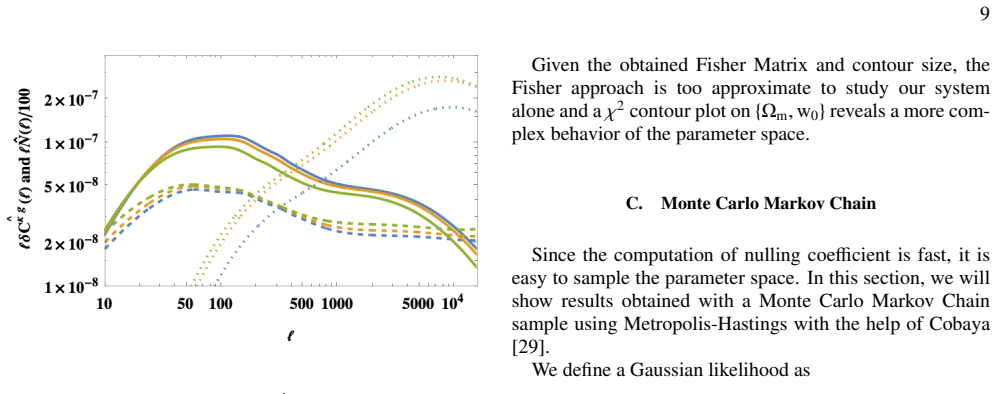
[Fig. 3 and §V.A] The text says the noise is divided by 100 ≈ √10,000 because roughly 10,000 ℓ modes are available. Since the analysis uses 32 logarithmically spaced ℓ bins, the effective mode count is an integral of (2ℓ+1) f_sky over each bin, not a single factor of 10,000. Please clarify how the scaled noise amplitude is defined.
[§VI.C] The diagonalization of the Fisher matrix is used to identify exact degeneracy directions, e.g., a 'kernel of dimension 3'. Fisher eigenvalues identify approximate null directions at a given fiducial model; the language should be softened unless an exact algebraic proof is intended.
[Tables I and II] The posteriors in Figs. 6–9 are visibly non-Gaussian; reporting the maximum-a-posteriori point and credible intervals in addition to the marginal one-sigma ranges would make the quoted intervals easier to interpret.

Circularity Check

0 steps flagged · score 0.0 of 10

No significant circularity: nulling coefficients are computed from assumed geometry and tested against measured cross-spectra; the target parameters are not fitted to the nulled spectra.

full rationale

The derivation is self-contained and non-circular. The nulling coefficients pai(θ) are computed from the assumed background geometry through the moments n_i^(1)(θ)=∫dχ n_i(χ)/FK(χ) (Eqs. 7-12), and the nulled cross-spectra Ĉ^κg_ai=pa_j(θ)C̃^κg_ji are formed from measured source-lens cross-spectra. The likelihood (Eq. 50) compares these nulled spectra to zero (up to the Q3 bispectrum template), so Ωm and w0 enter only through the transform coefficients, not as parameters fitted to the nulled spectra themselves; wrong cosmologies produce nonzero residuals that are not fitted away. The covariance matrix (Eq. 27) is a noise model and does not define the signal. The Q3 marginalization absorbs a single amplitude of the bispectrum bias; any shape mismatch is a modeling approximation and a potential bias, not a circular reduction. Self-citations to the BNT transform literature are not load-bearing because Section II.A re-derives the nulling conditions and Appendix B proves the degeneracy. No circular step can be exhibited.

Assumptions & free parameters 2 free parameters · 7 assumptions · 0 invented entities

The central claim rests on a set of standard cosmological approximations and on the BNT construction from prior work; no new physical entities are introduced. The forecast depends on the nuisance parameter Q3 and on the photometric redshift error parameters z_b. The axioms are standard tools in weak lensing forecasts, but the single-Q3 bispectrum template and the Knox covariance are the most consequential choices.

free parameters (2)

Q3 = 1 (fiducial), marginalized
Nuisance parameter introduced to absorb the bispectrum bias from reduced shear and magnification bias (Eq. 45). It is a single scale-independent amplitude, which may not capture the full scale/redshift dependence of the bispectrum.
z_b (10 parameters) = 0 (fiducial), with Gaussian priors of width 10^-2 to 0 in different runs
Mean photometric redshift errors for the 10 source bins, added in Section VI. They are not the target of the probe but are essential systematics; the paper shows the null test is sensitive to them at the 10^-3 level.

assumptions (7)

domain assumption BNT nulling construction from Bernardeau et al. (2014), giving coefficients p_{ai} from the moments n^(0)_i and n^(1)_i (Eqs. 5-9).
The existence and form of the nulling coefficients are taken from [8]; the paper does not re-derive the general construction, only the explicit solution for equal-population bins (Eqs. 11-12).
domain assumption Limber approximation for all power spectra and correlators.
Stated in Section II.C: 'All along this paper, the correlators are computed in the context of the Limber approximation.' It also reduces some second-order terms to zero in Section IV.C.
domain assumption Pre-factor unity approximation, gamma_i = T_alpha(ell) kappa_i(ell).
Used in Eq. (35) to relate shear and convergence in the E-mode calculation; justified by references [25, 26] as negligible for Euclid-like surveys.
domain assumption Halofit non-linear matter power spectrum (Takahashi et al. 2012) with Planck best-fit parameters.
Used to compute the expected signal and covariance in Section II.C. The null test itself is independent of this modeling, but the forecast precision depends on it.
domain assumption Bispectrum fitting formula with a single amplitude Q3: B(k1,k2,k3) = Q3 [P(k1)P(k2) + cyc.] (Eq. 43).
Assumes the reduced-shear and magnification corrections have the shape of the gravitational bispectrum with a single normalization. This is the weakest modeling assumption and is used in Eq. (45) and the likelihood (Eq. 50).
domain assumption Knox (Gaussian) covariance with no super-sample covariance and no connected non-Gaussianities (Eq. 27).
Justified by the non-overlap of nulled kernels and low-redshift galaxy bins, which kills connected terms. This keeps the forecast independent of matter clustering details but relies on the binning scheme working as designed.
domain assumption The optimized low-redshift binning scheme ensures residual overlap below 1% of the signal.
Section III.A.2 and Appendix C choose bin limits so that the product of nulled kernels and galaxy distributions is below 1% of the maximum non-nulled signal, allowing the null condition to be treated as exact within noise.

how reviews work

0 comments

Cite this review

Pith. "Pith review of Cosmic shear nulling as a geometrical cosmological probe: Methodology and sensitivity to cosmological parameters and systematics." pith.science (2026). https://pith.science/paper/3Y6DFUN3

@misc{pith2026250202246,
  author       = {Pith},
  title        = {Pith review of: Cosmic shear nulling as a geometrical cosmological probe: Methodology and sensitivity to cosmological parameters and systematics},
  year         = {2026},
  howpublished = {\url{https://pith.science/paper/3Y6DFUN3}},
  note         = {Machine review of arXiv:2502.02246}
}

abstract

Tomographic weak lensing surveys contain intrinsic symmetries that depend solely on the geometric structure of the Universe. These symmetries can be revealed through null tests and verifying their validity provides constraints on cosmological parameters that govern the background evolution-particularly the redshift dependence of the angular diameter distance. This forms the foundation of the tomographic cosmic shear nulling test introduced in this work. We describe how this test can be implemented, what aspects of cosmology it can constrain, and its specific efficiency in doing so. We also assess its sensitivity to astrophysical effects-such as magnification bias and reduced shear corrections-as well as to observational systematics, including errors in the mean redshift of source bins. Our results show that, in a survey configuration comparable to that of Euclid, this null test can yield complementary constraints on key cosmological parameters such as ${\Omega_{\rm m}, {\rm w}_0}$. However, due to its subdominant constraining power compared to standard 3x2pt analysis and through the identification of a required precision of order $10^{-3}$ on the mean redshift of the bins, we conclude that nulling would better be used as a photometric redshift calibration probe or consistency check. In combination with standard weak lensing and galaxy clustering analysis, it would then offer a promising route to better control systematics and improve the precision of future cosmological measurements.

Figures

Figures reproduced from arXiv: 2502.02246 by the authors.

**Figure 1.** Shape of the nulled lensing kernels ˆwa(z) (solid lines) and of the original lensing kernels wi(z) (dashed lines), as constructed for 10 tomographic bins and a photometric redshift uncertainty σz = 0.02. As an illustration, [PITH_FULL_IMAGE:figures/full_fig_p003_1.png] view at source ↗

**Figure 2.** 8-th nulled lensing kernel (blue solid line) and low [PITH_FULL_IMAGE:figures/full_fig_p004_2.png] view at source ↗

**Figure 3.** Amplitude of the signal ℓδC κˆg (ℓ) (solid lines) for a 10% variation of w0 and noise level ℓNˆ(ℓ)/100 (dashed lines) both for σz = 0 (blue), 0.02 (yellow), 0.05 (green) as a function of ℓ. We show as an example in [PITH_FULL_IMAGE:figures/full_fig_p008_3.png] view at source ↗

Figures from the paper (7 more)

**Figure 4.** Figure 4: Amplitude of the signal ℓδC κˆg (ℓ) (solid lines) for a 10% variation of w0 and noise level ℓNˆ(ℓ)/100 (dashed lines) both for σz = 0 (blue), 0.02 (yellow), 0.05 (green) as functions of ℓ. The dotted lines represent the effective amplitudes δBC κˆg (ℓ) for the same val…

**Figure 5.** Figure 5: Gaussian contour at 1σ obtained with the Fisher approach without bispectrum corrections (dashed) and marginalising over Q3 (solid lines) with σz = 0.02. We show in [PITH_FULL_IMAGE:figures/full_fig_p009_5.png]

**Figure 6.** Figure 6: Posterior distribution for Ωm with sampled parameters {Ωm, w0, Q3}. We show different cases of fixed parameters. In green: {w0, Q3} are fixed. In blue: w0 is fixed. In red: Q3 is fixed [PITH_FULL_IMAGE:figures/full_fig_p010_6.png]

**Figure 8.** Figure 8: χ 2 contour plot for {Ωm, w0} marginalised over Q3 in blue. Degeneracy lines at fixed redshifts, indicated next to the curves, in orange. The reference model for these lines is {Ωm = 0.30, w0 = −0.95}. We then investigate the evolution of performances for different ma…

**Figure 7.** Figure 7: Triangle plot for sampled parameters {Ωm, w0, Q3}. Dashed lines show the fiducial values of parameters. However, let us emphasize that the nulling test is still adding constraints on the parameters as this correlation is not the same as in usual weak lensing analysis. …

**Figure 9.** Figure 9: Evolution of the triangle plot for sampled parameters [PITH_FULL_IMAGE:figures/full_fig_p011_9.png]

**Figure 10.** Figure 10: Evolution of the triangle plot for sampled parame [PITH_FULL_IMAGE:figures/full_fig_p012_10.png]

Discussion (0). Continue with ORCID to comment.

Forward citations

Cited by 1 Pith paper

Reviewed papers in the Pith corpus that reference this work. Sorted by Pith novelty score. Full citation record

Mitigating Nonlinear Systematics in Weak Lensing Surveys: The Bernardeau-Nishimichi-Taruya Approach
astro-ph.CO 2024-12 conditional novelty 5.0 of 10

The BNT transform of cosmic shear data makes ℓ-space cuts behave like k-space cuts, reducing nonlinear scale leakage and preserving unbiased S8 constraints in Euclid-like forecasts.

Reference graph

Works this paper leans on

40 extracted references · 12 canonical work pages · cited by 1 Pith paper

[1]

Source galaxies For the sources, we work with 10 equally populated red- shift bins as in [22], each having a galaxy surface density of ni = 3 arcmin−2, in the intervals (with sorted zi): {0.0010, 0.42, 0.56, 0.68, 0.79, 0.90, 1.02, 1.15, 1.32, 1.58, 2.50}. We then define the normalized redshift distribution of galaxies in the i-th bin as ni(z) = R zi+1 zi...

work page
[2]

One simple solution for low redshift galaxy distributions is to use the same specification as for sources

Low Redshift Galaxies Let us now turn to the binned low redshift galaxy density fields which are defined as δg i (n) = Z ∞ 0 dχ ng i (χ)δm(χ, n), (19) where ng i are binned redshift4 galaxy distributions which we describe in this section. One simple solution for low redshift galaxy distributions is to use the same specification as for sources. However, wh...

work page
[3]

The binning is opti- mized for different values of the photometric redshift uncer- taintyσz

Results The resulting bin limits for the low redshift galaxy dis- tributions are summarized in Table III. The binning is opti- mized for different values of the photometric redshift uncer- taintyσz. Table III. Low redshift galaxy bin limits. Source σz = 0 σz = 0.02 σz = 0.05 0.001 zg(1) 0 .001 0 .001 0 .001 0.417733 zg(2) 0 .461323 0 .415625 0 .329181 0.5...

work page
[4]

T. M. C. Abbott et al. (DES), Dark Energy Survey Year 3 results: Cosmological constraints from galaxy cluster- ing and weak lensing, Phys. Rev. D 105, 023520 (2022), arXiv:2105.13549 [astro-ph.CO]

arXiv 2022
[5]

(A2) For simplicity, we will drop the tilde in the main text

Fourier Transform In this paper, we use the following conventions for n- dimensional Fourier transforms ˜f (k) = 1√(2π)n Z dnxe−ik·x f (x), (A1) f (x) = 1√(2π)n Z dnkeik·x ˜f (k). (A2) For simplicity, we will drop the tilde in the main text. The variables we will use will be n for the 2-dimensional unit less position in sky and ℓ for the corresponding sca...

work page
[6]

Polyspectra Normalizations We use the following conventions for the spectrum and bispectrum. a. Spectrum and 2-point correlation functions: D˜δm(k)˜δm(k′) E =δD(k + k′)P(k) (A3) ⟨δm(x)δm(x + r)⟩ = Z d3k (2π)3 P(k)eik.r (A4) σ2 = D δ2 m E =ξ(0) = Z d3k (2π)3 P(k) (A5) dσ2 dlnk = 4πk3 (2π)3 P(k) (A6) b. Bispectrum: D˜δm(k1)˜δm(k2)˜δm(k3) E = 1p (2π)3 δD(k1 ...

work page
[7]

Methodology To ensure that the nulled lensing kernel ˆ wa(z) and the galaxy distribution na−3(z) meet the 10% threshold, we de- fine two key redshifts:

work page
[8]

This procedure is purely geometri- cal and thus scale-independent and independent of the power spectrum or matter density contrast

introduced nulling as a technique to build linear com- binations of cosmic shear maps that are only sensitive to a restricted redshift range. This procedure is purely geometri- cal and thus scale-independent and independent of the power spectrum or matter density contrast. It can be thought of as a way to reorganise the information contained in cosmic she...

work page

Show all 40 references

[9]

Specifically, we require ˆwa(z) ⩽ 0.1× max( ˆwa(z))≈ 0.02 for z ⩽ z ˆw(a), where we take 0.2 as an approximated common maximum value across all nulled lensing kernels

The redshift z ˆw(a), defined as the redshift below which the nulled lensing kernel ˆwa(z) remains less than 10% of its maximum value. Specifically, we require ˆwa(z) ⩽ 0.1× max( ˆwa(z))≈ 0.02 for z ⩽ z ˆw(a), where we take 0.2 as an approximated common maximum value across al...
[10]

Specifically, we require na−3(z ˆw(a)) ⩽ 0.1× n(z), to ensure that the overlap between na−3(z) and ˆwa(z) con- tributes negligibly to the signal

The photometric redshift zg(a− 3), defined as the red- shift where the galaxy bin is cut to ensure that the galaxy number density na−3 is sufficiently small at z ˆw(a) and higher redshifts. Specifically, we require na−3(z ˆw(a)) ⩽ 0.1× n(z), to ensure that the overlap between ...
[11]

Implementation Details The bin limits zg(i) are chosen to meet the following con- ditions: zg(1) = zmin, zg(i ⩾ 8) = zi, fi(z ˆw(i + 3)) = 0.1 for i ⩽ 7. where fi(z) = R zg(i+1) zg(i) dzp pph(zp, z,σ z, zi b = 0) is the fraction of galaxies at real redshift z that are labeled ...
[12]

J. T. A. de Jong, G. A. Verdoes Kleijn, K. H. Kuijken, and E. A. Valentijn (Astro-WISE, KiDS), The Kilo-Degree Sur- vey, Exper. Astron. 35, 25 (2013), arXiv:1206.1254 [astro- ph.CO]

2013 arXiv
[13]

Asgari et al

M. Asgari et al. (KiDS), KiDS-1000 Cosmology: Cosmic shear constraints and comparison between two point statis- tics, Astron. Astrophys. 645, A104 (2021), arXiv:2007.15633 [astro-ph.CO]

2021 arXiv
[14]

Abbott et al

T. Abbott et al. (DES), The Dark Energy Survey, (2005), arXiv:astro-ph/0510346

2005 arXiv
[15]

pre-factor unity approximation

can be identified to local nulling techniques described in [13]. The reasoning is as follows: if the low redshift galaxy distributions are narrow enough, then the ratios qi, j,k(ℓ) = Cκg ji (ℓ) Cκg ki (ℓ) (28) are constant and depend only on the background geometry of space-ti...
[16]

Abate et al

A. Abate et al. (LSST Dark Energy Science), Large Synop- tic Survey Telescope: Dark Energy Science Collaboration, (2012), arXiv:1211.0310 [astro-ph.CO]

2012 arXiv
[17]

Mellier et al

Y . Mellier et al. (Euclid), Euclid. I. Overview of the Euclid mission, (2024), arXiv:2405.13491 [astro-ph.CO]

2024
[18]

Hu, Power spectrum tomography with weak lensing, As- trophys

W. Hu, Power spectrum tomography with weak lensing, As- trophys. J. Lett. 522, L21 (1999), arXiv:astro-ph/9904153

1999 arXiv
[19]

Bernardeau, T

F. Bernardeau, T. Nishimichi, and A. Taruya, Cosmic shear full nulling: sorting out dynamics, geometry and sys- tematics, Mon. Not. Roy. Astron. Soc. 445, 1526 (2014), arXiv:1312.0430 [astro-ph.CO]

2014 arXiv
[20]

P. L. Taylor, F. Bernardeau, and E. Huff, x-cut Cosmic Shear: Optimally Removing Sensitivity to Baryonic and Nonlin- ear Physics with an Application to the Dark Energy Sur- 17 vey Year 1 Shear Data, Phys. Rev. D 103, 043531 (2021), arXiv:2007.00675 [astro-ph.CO]

2021 arXiv
[21]

Bernardeau, T

F. Bernardeau, T. Nishimichi, and A. Taruya, Observing Bary- onic Acoustic Oscillations in tomographic cosmic shear sur- veys, (2020), arXiv:2004.03201 [astro-ph.CO]

2020 arXiv
[22]

Fronenberg, A

H. Fronenberg, A. S. Maniyar, A. R. Pullen, and A. Liu, Con- straining Cosmology With the CMB× LIM-Nulling Conver- gence, (2023), arXiv:2309.06477 [astro-ph.CO]

2023 arXiv
[23]

A. S. Maniyar, E. Schaan, and A. R. Pullen, New probe of the high-redshift Universe: Nulling CMB lensing with interloper- free line intensity mapping pair lensing, Phys. Rev. D 105, 083509 (2022), arXiv:2106.09005 [astro-ph.CO]

2022 arXiv
[24]

Joachimi and P

B. Joachimi and P. Schneider, Controlling intrinsic alignments in weak lensing statistics: The nulling and boosting tech- niques, (2010), arXiv:1009.2024 [astro-ph.CO]

2010 arXiv
[25]

Prat et al

J. Prat et al. (DES, SPT), Cosmological lensing ratios with DES Y1, SPT and Planck, Mon. Not. Roy. Astron. Soc. 487, 1363 (2019), arXiv:1810.02212 [astro-ph.CO]

2019 arXiv
[26]

Sánchez et al

C. Sánchez et al. (DES), Dark Energy Survey Year 3 results: Exploiting small-scale information with lensing shear ratios, Phys. Rev. D 105, 083529 (2022), arXiv:2105.13542 [astro- ph.CO]

2022 arXiv
[27]

E. Abdalla et al., Cosmology intertwined: A review of the par- ticle physics, astrophysics, and cosmology associated with the cosmological tensions and anomalies, JHEAp 34, 49 (2022), arXiv:2203.06142 [astro-ph.CO]

2022 arXiv
[28]

Tutusaus et al

I. Tutusaus et al. (EUCLID), Euclid: The importance of galaxy clustering and weak lensing cross-correlations within the photometric Euclid survey, Astron. Astrophys. 643, A70 (2020), arXiv:2005.00055 [astro-ph.CO]

2020 arXiv
[29]

Kaiser, Weak gravitational lensing of distant galaxies, As- trophys

N. Kaiser, Weak gravitational lensing of distant galaxies, As- trophys. J. 388, 272 (1992)

1992
[30]

Takahashi, M

R. Takahashi, M. Sato, T. Nishimichi, A. Taruya, and M. Oguri, Revising the Halofit Model for the Nonlinear Matter Power Spectrum, Astrophys. J. 761, 152 (2012), arXiv:1208.2701 [astro-ph.CO]

2012 arXiv
[31]

R. E. Smith, J. A. Peacock, A. Jenkins, S. D. M. White, C. S. Frenk, F. R. Pearce, P. A. Thomas, G. Efstathiou, and H. M. P. Couchmann (VIRGO Consortium), Stable clustering, the halo model and nonlinear cosmological power spectra, Mon. Not. Roy. Astron. Soc. 341, 1311 (2003), ...

2003 arXiv
[32]

Aghanim et al

N. Aghanim et al. (Planck), Planck 2018 results. I. Overview and the cosmological legacy of Planck, Astron. Astrophys. 641, A1 (2020), arXiv:1807.06205 [astro-ph.CO]

2020 arXiv
[33]

Blanchard et al

A. Blanchard et al. (Euclid), Euclid preparation. VII. Forecast validation for Euclid cosmological probes, Astron. Astrophys. 642, A191 (2020), arXiv:1910.09273 [astro-ph.CO]

2020 arXiv
[34]

A. C. Deshpande et al. , Euclid: The reduced shear ap- proximation and magnification bias for Stage IV cosmic shear experiments, Astron. Astrophys. 636, A95 (2020), arXiv:1912.07326 [astro-ph.CO]

2020 arXiv
[35]

Knox, Determination of inflationary observables by cosmic microwave background anisotropy experiments, Phys

L. Knox, Determination of inflationary observables by cosmic microwave background anisotropy experiments, Phys. Rev. D 52, 4307 (1995), arXiv:astro-ph/9504054

1995 arXiv
[36]

T. D. Kitching, J. Alsing, A. F. Heavens, R. Jimenez, J. D. McEwen, and L. Verde, The Limits of Cosmic Shear, Mon. Not. Roy. Astron. Soc. 469, 2737 (2017), arXiv:1611.04954 [astro-ph.CO]

2017 arXiv
[37]

Kilbinger et al., Precision calculations of the cosmic shear power spectrum projection, Mon

M. Kilbinger et al., Precision calculations of the cosmic shear power spectrum projection, Mon. Not. Roy. Astron. Soc.472, 2126 (2017), arXiv:1702.05301 [astro-ph.CO]

2017 arXiv
[38]

F. J. Castander et al. (Euclid), Euclid. V . The Flagship galaxy mock catalogue: a comprehensive simulation for the Euclid mission, (2024), arXiv:2405.13495 [astro-ph.CO]

2024
[39]

Scoccimarro and H

R. Scoccimarro and H. M. P. Couchman, A fitting formula for the nonlinear evolution of the bispectrum, Mon. Not. Roy. Astron. Soc. 325, 1312 (2001), arXiv:astro-ph/0009427

2001 arXiv
[40]

Torrado and A

J. Torrado and A. Lewis, Cobaya: Code for Bayesian Analysis of hierarchical physical models, JCAP 05, 057, arXiv:2005.05290 [astro-ph.IM]

2005 arXiv

Pith tools

Reviewed August 9, 2026 · model on record in the stance chip above.

[1] [1]

Source galaxies For the sources, we work with 10 equally populated red- shift bins as in [22], each having a galaxy surface density of ni = 3 arcmin−2, in the intervals (with sorted zi): {0.0010, 0.42, 0.56, 0.68, 0.79, 0.90, 1.02, 1.15, 1.32, 1.58, 2.50}. We then define the normalized redshift distribution of galaxies in the i-th bin as ni(z) = R zi+1 zi...

work page

[2] [2]

One simple solution for low redshift galaxy distributions is to use the same specification as for sources

Low Redshift Galaxies Let us now turn to the binned low redshift galaxy density fields which are defined as δg i (n) = Z ∞ 0 dχ ng i (χ)δm(χ, n), (19) where ng i are binned redshift4 galaxy distributions which we describe in this section. One simple solution for low redshift galaxy distributions is to use the same specification as for sources. However, wh...

work page

[3] [3]

The binning is opti- mized for different values of the photometric redshift uncer- taintyσz

Results The resulting bin limits for the low redshift galaxy dis- tributions are summarized in Table III. The binning is opti- mized for different values of the photometric redshift uncer- taintyσz. Table III. Low redshift galaxy bin limits. Source σz = 0 σz = 0.02 σz = 0.05 0.001 zg(1) 0 .001 0 .001 0 .001 0.417733 zg(2) 0 .461323 0 .415625 0 .329181 0.5...

work page

[4] [4]

T. M. C. Abbott et al. (DES), Dark Energy Survey Year 3 results: Cosmological constraints from galaxy cluster- ing and weak lensing, Phys. Rev. D 105, 023520 (2022), arXiv:2105.13549 [astro-ph.CO]

arXiv 2022

[5] [5]

(A2) For simplicity, we will drop the tilde in the main text

Fourier Transform In this paper, we use the following conventions for n- dimensional Fourier transforms ˜f (k) = 1√(2π)n Z dnxe−ik·x f (x), (A1) f (x) = 1√(2π)n Z dnkeik·x ˜f (k). (A2) For simplicity, we will drop the tilde in the main text. The variables we will use will be n for the 2-dimensional unit less position in sky and ℓ for the corresponding sca...

work page

[6] [6]

Polyspectra Normalizations We use the following conventions for the spectrum and bispectrum. a. Spectrum and 2-point correlation functions: D˜δm(k)˜δm(k′) E =δD(k + k′)P(k) (A3) ⟨δm(x)δm(x + r)⟩ = Z d3k (2π)3 P(k)eik.r (A4) σ2 = D δ2 m E =ξ(0) = Z d3k (2π)3 P(k) (A5) dσ2 dlnk = 4πk3 (2π)3 P(k) (A6) b. Bispectrum: D˜δm(k1)˜δm(k2)˜δm(k3) E = 1p (2π)3 δD(k1 ...

work page

[7] [7]

Methodology To ensure that the nulled lensing kernel ˆ wa(z) and the galaxy distribution na−3(z) meet the 10% threshold, we de- fine two key redshifts:

work page

[8] [8]

This procedure is purely geometri- cal and thus scale-independent and independent of the power spectrum or matter density contrast

introduced nulling as a technique to build linear com- binations of cosmic shear maps that are only sensitive to a restricted redshift range. This procedure is purely geometri- cal and thus scale-independent and independent of the power spectrum or matter density contrast. It can be thought of as a way to reorganise the information contained in cosmic she...

work page