REVIEW 4 major objections 4 minor 45 references
Loss Landscape Analysis for Reliable Quantized ML Models for Scientific Sensing
T0 review · 4 major / 4 minor · reviewed 2026-08-08 · deepseek-v4-flash
Pith's one-line read The paper claims that a quantized model's robustness to noise and bit flips can be predicted from the shape of its loss landscape before any perturbation testing.
desk verdict Useful observational study, but the a priori robustness claim is in-sample and unquantified. read the letter →
The pith
A machine-rendered reading of the paper's core claim, the machinery that carries it, and where it could break.
The reading
What carries the argument
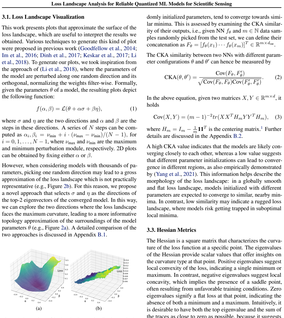
The machinery is a set of loss-landscape metrics computed at the end of quantization-aware training. CKA similarity measures whether independent trainings converge to similar output representations; Hessian trace, approximated by power iteration, measures local curvature at the minimum; mode connectivity, computed along a trained Bezier curve between two minima, measures the height of loss barriers separating them; and 2D projections along the top-2 eigenvectors of the Hessian visualize the landscape in its most curved directions. The paper uses these four measurements together to rank model configurations by expected robustness.
What would settle it
Train a third family of quantized models (for example a larger CNN or a small transformer) across the same bit widths and regularizers; if any configuration with lower Hessian trace and lower mode-connectivity barriers than its peers still degrades more under Gaussian noise or top-5 bit flips, the claimed correlation fails for that family. A direct test: compute the metrics on one seed and rank configurations, then blind-test robustness on held-out seeds; a mismatch between predicted and observed ranking would refute the a priori claim.
Extended reading notes
Core claim
The discovery the paper argues for is a correlation between loss-landscape geometry and robustness in quantized scientific-sensing models: configurations whose converged loss landscape is flatter locally (lower Hessian trace), more connected globally (fewer barriers along Bezier paths between minima), and more consistent across random initializations (higher CKA similarity) tend to degrade less under Gaussian input noise, salt-and-pepper noise, and flips of the most sensitive weight bits. The same metrics explain why regularization helps one model and not the other, and why reducing bit width sometimes improves robustness: low-bit quantization acts as an implicit regularizer that flattens the landscape. The paper's further claim is that these metrics can be computed on converged models and used to rank configurations before any perturbation testing, so robustness can enter model search without extra training campaigns.
Load-bearing premise
The load-bearing premise is that loss-landscape geometry measured on clean, converged models predicts robustness to perturbations never used in training, and that this holds beyond the two model families and the Gaussian, salt-and-pepper, and sensitive-bit-flip tests studied here.
Editorial extensions
If this is right
- Designers can screen candidate quantized configurations by computing landscape metrics once, instead of running noise-injection and bit-flip campaigns for every setting.
- Robustness can be added as a third axis in Pareto optimization alongside accuracy and efficiency, since the metrics are available before deployment.
- Low-bit quantization should not be assumed to harm robustness; the landscape metrics identify cases where it flattens the loss and improves resilience.
- The choice of regularizer is model-dependent: the same regularizer that flattens one model's landscape can steepen another's, and landscape metrics reveal which.
- Because the method is agnostic to the perturbation source, insights transfer to unknown corruptions encountered in the field.
Reading between the lines
- If the correlation generalizes, the same metrics could be used as a training signal or early-stopping criterion, for example penalizing Hessian trace during quantization-aware training to actively steer models toward robust minima; the paper does not test this.
- The paper's evidence is limited to two small models and three perturbation types; a natural test is whether the ordering holds for larger architectures or for adversarial and domain-shift corruptions.
- The gentle-landscape notion could connect to a quantitative robustness certificate: a bound on loss change under bounded weight perturbations in terms of Hessian trace and mode-connectivity barrier height, something the paper only hints at.
- For the scientific-sensing community, the practical payoff would be a deployment checklist: quantize, compute three numbers, and pick the configuration with the flattest trace and lowest barriers, before burning FPGA synthesis time.
Editorial analysis
A structured set of objections, weighed in public.
Referee Report
Summary. The paper proposes a loss-landscape analysis method for quantized ML models used in scientific sensing, combining top-eigenvector-based visualization, CKA similarity, Hessian trace, and mode connectivity. It applies this method to two real-world-inspired models (ECON-T and Fusion) under baseline, Jacobian, and orthogonal regularization across precision levels, and compares the landscape metrics with robustness to Gaussian noise, salt-and-pepper noise, and FKeras-ranked bit flips. The headline claim is that gently shaped loss landscapes are strongly correlated with robustness, enabling a priori identification of robust configurations without training and testing campaigns. The central empirical claim is plausible and well-motivated, but the current evidence is weakened by an in-sample selection step, the absence of a quantitative correlation measure, and the lack of a genuine held-out prediction test.
Significance. If validated, the ability to screen quantized model configurations for robustness to input noise and weight perturbations using only loss landscape metrics would be a valuable design-time tool for edge scientific sensing, where exhaustive brute-force testing is costly. The paper addresses an important and underexplored reliability dimension of quantization, releases code, and uses two deployment-inspired models with practically relevant corruption models. These strengths make the work worth pursuing, but the significance is conditional: the claimed a priori predictive power is currently inferred from post-hoc, in-sample agreement, not demonstrated by a prediction exercise.
major comments (4)
- [Appendix C.2; Section 5.2] The a priori predictive claim is not actually tested for the Fusion model. The authors state in Appendix C.2 that they 'tested different values of δ and selected the one that provided the best trade-off' on clean and 10% Gaussian-perturbed inputs, choosing δ = 1e-6 for both regularizers; these same configurations are then used in the main robustness comparison in Section 5.2. Any agreement between the landscape metrics in Figures 4b, 4d, 4f and the robustness results in Figures 5f, 5g, 5h is therefore an in-sample correlation, not an out-of-sample prediction. Please add a genuinely held-out evaluation: pre-specify a configuration grid, compute the landscape metrics, and then test robustness for perturbation types, noise magnitudes, or precision levels not used in any tuning step.
- [Section 5.1; Section 5.2; Figures 4 and 5] The claimed 'strong correlation' between loss landscape metrics and robustness is supported only by visual matching of Figures 4 and 5. No quantitative correlation coefficient, rank correlation, or confidence interval is reported, and the results from the three training seeds are averaged without error bars. Please report a quantitative association (e.g., Spearman correlation) between each landscape metric (CKA, Hessian trace, mode connectivity) and each robustness outcome across the full set of configurations, together with per-seed variability, so that the strength and stability of the claimed correlation can be assessed.
- [Section 6; Impact Statement] The conclusion and impact statement generalize to 'unknown corruptions' and 'out-of-training-distribution corruptions,' but the experiments cover only Gaussian noise, salt-and-pepper noise, and flipping the five most FKeras-sensitive bits on two model families. This generalization is load-bearing for the practical workflow, because the a priori value would be to avoid benchmarking unseen corruptions. Please either test at least one additional corruption type or severity not used in any earlier step, or explicitly restrict the claims to the perturbation families studied.
- [Section 3.1; Appendix B.1] The method assumes that the top-2 eigenvectors of the model parameters provide a representative 2D slice of the loss landscape. The ablation in Figure 7 demonstrates only that random directions produce a different scale; it does not validate that the top-2 slice captures the geometry relevant to robustness. Since the visualization is used to support the qualitative interpretation, this assumption should be justified or its influence on the conclusions examined, even though the quantitative metrics (CKA, Hessian trace, mode connectivity) do not depend on this particular choice.
minor comments (4)
- [Figure 3] The loss-curve panels lack axis labels for the perturbation magnitude and loss value; adding shared labels and reporting the evaluation range in the caption would make the comparison easier to interpret.
- [Section 5.1, Figure 4] The text refers to 'inset (c)' and 'inset (d)' for the Hessian trace panels, but the figures do not appear to contain actual insets; either add insets or rephrase the reference.
- [Section 3.2] The CKA metric is computed with m = 10 concatenated outputs based on the ablation in Figure 7a; a brief statement of how stable the reported figures are to this choice would be useful, since the ablation shows sensitivity to m.
- [Section 5.2] The paper states that 'for most configurations, except for extreme low-bit settings (e.g., 3 or 4 bits) ... these phenomena are strongly correlated,' but does not specify which metric is being correlated with which robustness outcome; please make the intended pairing explicit.
Circularity Check
Regularization strengths are tuned on the perturbation benchmark, so the 'a priori' landscape-robustness correlation is in-sample for the Fusion model.
-
fitted input called prediction
[Appendix C.2 (Figs. 9a-9d) and Section 5 (Eqs. (6)-(7), Figs. 4-5)]
"In this study, we tested different values of δ and selected the one that provided the best trade-off (δ = 10−6 in this case). ... Fine-tuning this trade-off often requires several iterations to test various noise types and magnitudes to guarantee reliability."
The chosen δ = 10−6 is used for both Jacobian and orthogonal regularization on the Fusion model in Section 5, and Appendix C.2 selected it by evaluating models on clean data and on 10% Gaussian-perturbed inputs (Figs. 9a-9d). The Fusion configurations whose CKA similarity, Hessian trace, and mode connectivity are said to align with robustness were therefore selected using the Gaussian perturbation benchmark that the landscape metrics are claimed to predict a priori.
full rationale
This is a partial, protocol-level circularity rather than an equation-level one. The loss-landscape metrics themselves are computed by standard external definitions, and the FKeras bit-flip benchmark is independently validated against random flips in Appendix C.1, so no self-citation chain or imported uniqueness theorem is load-bearing. However, the paper's central 'a priori' claim is not actually tested even for the studied cases: the Fusion regularization strengths used in the main comparison were tuned on the 10% Gaussian-noise benchmark, making the subsequent landscape-robustness agreement partly in-sample. The claimed 'strong correlation' is also supported only by visual alignment between Figures 4 and 5, with no quantitative correlation measure, which compounds the problem but is not itself circularity. The score reflects that one central claim reduces to a selection fitted to the outcome, while the underlying empirical correlation retains some independent content.
Assumptions & free parameters
free parameters (4)
- Jacobian regularization weight delta (ECON-T) =
0.1
- Jacobian regularization weight delta (Fusion) =
1e-6
- Orthogonal regularization weight delta (ECON-T) =
1e-5
- Orthogonal regularization weight delta (Fusion) =
1e-6
assumptions (4)
- domain assumption Loss landscape geometry (flatness, connectivity, representational similarity) is a meaningful and measurable proxy for perturbation robustness.
- domain assumption PyHessian's power method approximates the Hessian trace accurately for these small models.
- ad hoc to paper The top-2 eigenvectors of model parameters provide a representative 2D slice of the loss landscape.
- domain assumption The FKeras sensitivity score ranks bit significance correctly for worst-case bit flips.
Cite this review
Pith. "Pith review of Loss Landscape Analysis for Reliable Quantized ML Models for Scientific Sensing." pith.science (2026). https://pith.science/paper/TISIT6QH
@misc{pith2026250208355,
  author       = {Pith},
  title        = {Pith review of: Loss Landscape Analysis for Reliable Quantized ML Models for Scientific Sensing},
  year         = {2026},
  howpublished = {\url{https://pith.science/paper/TISIT6QH}},
  note         = {Machine review of arXiv:2502.08355}
}
read the original abstract
In this paper, we propose a method to perform empirical analysis of the loss landscape of machine learning (ML) models. The method is applied to two ML models for scientific sensing, which necessitates quantization to be deployed and are subject to noise and perturbations due to experimental conditions. Our method allows assessing the robustness of ML models to such effects as a function of quantization precision and under different regularization techniques -- two crucial concerns that remained underexplored so far. By investigating the interplay between performance, efficiency, and robustness by means of loss landscape analysis, we both established a strong correlation between gently-shaped landscapes and robustness to input and weight perturbations and observed other intriguing and non-obvious phenomena. Our method allows a systematic exploration of such trade-offs a priori, i.e., without training and testing multiple models, leading to more efficient development workflows. This work also highlights the importance of incorporating robustness into the Pareto optimization of ML models, enabling more reliable and adaptive scientific sensing systems.
Figures


Figures from the paper (6 more)


Reference graph
Works this paper leans on
-
[1]
write newline
" write newline "" before.all 'output.state := FUNCTION n.dashify 't := "" t empty not t #1 #1 substring "-" = t #1 #2 substring "--" = not "--" * t #2 global.max substring 't := t #1 #1 substring "-" = "-" * t #2 global.max substring 't := while if t #1 #1 substring * t #2 global.max substring 't := if while FUNCTION format.date year duplicate empty "emp...
-
[2]
Can we gain more from orthogonality regularizations in training deep cnns? arxiv 2018
Bansal, N., Chen, X., and Wang, Z. Can we gain more from orthogonality regularizations in training deep cnns? arxiv 2018. arXiv preprint arXiv:1810.09102
arXiv 2018
-
[3]
Large scale gan training for high fidelity natural image synthesis
Brock, A. Large scale gan training for high fidelity natural image synthesis. arXiv preprint arXiv:1809.11096, 2018
arXiv 2018
-
[4]
Cheng, H., Zhang, M., and Shi, J. Q. A survey on deep neural network pruning: Taxonomy, comparison, analysis, and recommendations. IEEE Transactions on Pattern Analysis and Machine Intelligence, 2024
2024
-
[5]
Choromanska, A., Henaff, M., Mathieu, M., Arous, G. B., and LeCun, Y. The loss surfaces of multilayer networks. In Artificial intelligence and statistics, pp.\ 192--204. PMLR, 2015
work page 2015
-
[6]
Parseval networks: Improving robustness to adversarial examples
Cisse, M., Bojanowski, P., Grave, E., Dauphin, Y., and Usunier, N. Parseval networks: Improving robustness to adversarial examples. In International conference on machine learning, pp.\ 854--863. PMLR, 2017
2017
- [7]
-
[8]
B., Duarte, J., Gingu, C., Harris, P., Hirschauer, J., Kwok, M., Loncar, V., et al
Di Guglielmo, G., Fahim, F., Herwig, C., Valentin, M. B., Duarte, J., Gingu, C., Harris, P., Hirschauer, J., Kwok, M., Loncar, V., et al. A reconfigurable neural network asic for detector front-end data compression at the hl-lhc. IEEE Transactions on Nuclear Science, 68 0 (8): 0 2179--2186, 2021
work page 2021
Show all 45 references
-
[9]
Sharp minima can generalize for deep nets
Dinh, L., Pascanu, R., Bengio, S., and Bengio, Y. Sharp minima can generalize for deep nets. In International Conference on Machine Learning, pp.\ 1019--1028. PMLR, 2017
2017
-
[10]
Essentially no barriers in neural network energy landscape
Draxler, F., Veschgini, K., Salmhofer, M., and Hamprecht, F. Essentially no barriers in neural network energy landscape. In International conference on machine learning, pp.\ 1309--1318. PMLR, 2018
2018
-
[11]
Duarte, J., Tran, N., Hawks, B., Herwig, C., Muhizi, J., Prakash, S., and Reddi, V. J. FastML Science Benchmarks: Accelerating Real-Time Scientific Edge Machine Learning . In 5th Conference on Machine Learning and Systems , 7 2022
2022
-
[12]
H., and Hutter, F
Elsken, T., Metzen, J. H., and Hutter, F. Neural architecture search: A survey. Journal of Machine Learning Research, 20 0 (55): 0 1--21, 2019
2019
-
[13]
Eryilmaz, S. B. and Dundar, A. Understanding how orthogonality of parameters improves quantization of neural networks. IEEE Transactions on Neural Networks and Learning Systems, 34 0 (12): 0 10737--10746, 2022
2022
-
[14]
Deep ensembles: A loss landscape perspective
Fort, S., Hu, H., and Lakshminarayanan, B. Deep ensembles: A loss landscape perspective. arXiv preprint arXiv:1912.02757, 2019
1912 arXiv
-
[15]
K., Paul, M., Kharaghani, S., Roy, D
Fort, S., Dziugaite, G. K., Paul, M., Kharaghani, S., Roy, D. M., and Ganguli, S. Deep learning versus kernel learning: an empirical study of loss landscape geometry and the time evolution of the neural tangent kernel. Advances in Neural Information Processing Systems, 33: 0 5...
2020
-
[16]
P., and Wilson, A
Garipov, T., Izmailov, P., Podoprikhin, D., Vetrov, D. P., and Wilson, A. G. Loss surfaces, mode connectivity, and fast ensembling of dnns. Advances in neural information processing systems, 31, 2018
2018
-
[17]
W., and Keutzer, K
Gholami, A., Kim, S., Dong, Z., Yao, Z., Mahoney, M. W., and Keutzer, K. A survey of quantization methods for efficient neural network inference. In Low-Power Computer Vision, pp.\ 291--326. Chapman and Hall/CRC, 2022
2022
-
[18]
J., Vinyals, O., and Saxe, A
Goodfellow, I. J., Vinyals, O., and Saxe, A. M. Qualitatively characterizing neural network optimization problems. arXiv preprint arXiv:1412.6544, 2014
2014 arXiv
-
[19]
A., and Yaida, S
Hoffman, J., Roberts, D. A., and Yaida, S. Robust learning with jacobian regularization. arXiv preprint arXiv:1908.02729, 5 0 (6): 0 7, 2019
1908 arXiv
-
[20]
J., Tao, M., and Branson, K
Im, D. J., Tao, M., and Branson, K. An empirical analysis of deep network loss surfaces. ArXiv, abs/1612.04010, 2016. URL https://api.semanticscholar.org/CorpusID:13651606
2016 arXiv
-
[21]
Quantization and training of neural networks for efficient integer-arithmetic-only inference
Jacob, B., Kligys, S., Chen, B., Zhu, M., Tang, M., Howard, A., Adam, H., and Kalenichenko, D. Quantization and training of neural networks for efficient integer-arithmetic-only inference. In Proceedings of the IEEE conference on computer vision and pattern recognition, pp.\ 2...
2018
-
[23]
S., Mudigere, D., Nocedal, J., Smelyanskiy, M., and Tang, P
Keskar, N. S., Mudigere, D., Nocedal, J., Smelyanskiy, M., and Tang, P. T. P. On large-batch training for deep learning: Generalization gap and sharp minima, 2017. URL https://arxiv.org/abs/1609.04836
2017 arXiv
-
[24]
Similarity of neural network representations revisited
Kornblith, S., Norouzi, M., Lee, H., and Hinton, G. Similarity of neural network representations revisited. In International conference on machine learning, pp.\ 3519--3529. PMLR, 2019
2019
-
[25]
Adversarial machine learning at scale
Kurakin, A., Goodfellow, I., and Bengio, S. Adversarial machine learning at scale. arXiv preprint arXiv:1611.01236, 2016
2016 arXiv
-
[26]
Visualizing the loss landscape of neural nets
Li, H., Xu, Z., Taylor, G., Studer, C., and Goldstein, T. Visualizing the loss landscape of neural nets. Advances in neural information processing systems, 31, 2018
2018
-
[27]
Brecq: Pushing the limit of post-training quantization by block reconstruction
Li, Y., Gong, R., Tan, X., Yang, Y., Hu, P., Zhang, Q., Yu, F., Wang, W., and Gu, S. Brecq: Pushing the limit of post-training quantization by block reconstruction. arXiv preprint arXiv:2102.05426, 2021
2021 arXiv
-
[28]
Defensive quantization: When efficiency meets robustness
Lin, J., Gan, C., and Han, S. Defensive quantization: When efficiency meets robustness. arXiv preprint arXiv:1904.08444, 2019
1904 arXiv
-
[29]
Spectral normalization for generative adversarial networks
Miyato, T., Kataoka, T., Koyama, M., and Yoshida, Y. Spectral normalization for generative adversarial networks. arXiv preprint arXiv:1802.05957, 2018
2018 arXiv
-
[30]
A., Van Baalen, M., Louizos, C., and Blankevoort, T
Nagel, M., Amjad, R. A., Van Baalen, M., Louizos, C., and Blankevoort, T. Up or down? adaptive rounding for post-training quantization. In International Conference on Machine Learning, pp.\ 7197--7206. PMLR, 2020
2020
-
[31]
Do wide and deep networks learn the same things
Nguyen, T., Raghu, M., and Kornblith, S. Do wide and deep networks learn the same things. Uncovering How Neural Network Representations Vary with Width and Depth Cs. Lg: arXiv: 2010.15327, 2021
2010 arXiv
-
[32]
Xilinx/brevitas, 2023
Pappalardo, A. Xilinx/brevitas, 2023. URL https://doi.org/10.5281/zenodo.3333552
2023 doi
-
[33]
A comprehensive survey on model quantization for deep neural networks in image classification
Rokh, B., Azarpeyvand, A., and Khanteymoori, A. A comprehensive survey on model quantization for deep neural networks in image classification. ACM Trans. Intell. Syst. Technol., 14 0 (6), November 2023. ISSN 2157-6904. doi:10.1145/3623402. URL https://doi.org/10.1145/3623402
2023 doi
-
[34]
Rubner, Y., Tomasi, C., and Guibas, L. J. The Earth mover's distance as a metric for image retrieval. Int. J. Comput. Vis., 40: 0 99, 2000. doi:10.1023/A:1026543900054
-
[35]
Shenoy, R., Duarte, J., Herwig, C., Hirschauer, J., Noonan, D., Pierini, M., Tran, N., and Suarez, C. M. Differentiable earth mover’s distance for data compression at the high-luminosity lhc. Machine Learning: Science and Technology, 4 0 (4): 0 045058, 2023
2023
-
[36]
Sokolić, J., Giryes, R., Sapiro, G., and Rodrigues, M. R. D. Robust large margin deep neural networks. IEEE Transactions on Signal Processing, 65 0 (16): 0 4265--4280, 2017. doi:10.1109/TSP.2017.2708039
2017
-
[37]
The global landscape of neural networks: An overview
Sun, R., Li, D., Liang, S., Ding, T., and Srikant, R. The global landscape of neural networks: An overview. IEEE Signal Processing Magazine, 37 0 (5): 0 95--108, 2020
2020
-
[38]
and Ameen, S
Vadera, S. and Ameen, S. Methods for pruning deep neural networks. IEEE Access, 10: 0 63280--63300, 2022
2022
-
[39]
S., Ren, Y., Mahurin, E., Patel, C., Subramanian, S., Lee, S., Nagel, M., Soriaga, J., et al
van Baalen, M., Kuzmin, A., Nair, S. S., Ren, Y., Mahurin, E., Patel, C., Subramanian, S., Lee, S., Nagel, M., Soriaga, J., et al. Fp8 versus int8 for efficient deep learning inference. arXiv preprint arXiv:2303.17951, 2023
2023 arXiv
-
[40]
Wang, J., Chen, Y., Chakraborty, R., and Yu, S. X. Orthogonal convolutional neural networks. In Proceedings of the IEEE/CVF conference on computer vision and pattern recognition, pp.\ 11505--11515, 2020
2020
-
[41]
Qdrop: Randomly dropping quantization for extremely low-bit post-training quantization
Wei, X., Gong, R., Li, Y., Liu, X., and Yu, F. Qdrop: Randomly dropping quantization for extremely low-bit post-training quantization. arXiv preprint arXiv:2203.05740, 2022
2022 arXiv
-
[42]
F., Hansen, C., Levesque, J
Wei, Y., Forelli, R. F., Hansen, C., Levesque, J. P., Tran, N., Agar, J. C., Di Guglielmo, G., Mauel, M. E., and Navratil, G. A. Low latency optical-based mode tracking with machine learning deployed on FPGAs on a tokamak . Rev. Sci. Instrum., 95 0 (7): 0 073509, 2024. doi:10....
2024 doi
-
[43]
M., and Kastner, R
Weng, O., Meza, A., Bock, Q., Hawks, B., Campos, J., Tran, N., Duarte, J. M., and Kastner, R. Fkeras: A sensitivity analysis tool for edge neural networks. Journal on Autonomous Transportation Systems, 2024
2024
-
[44]
E., Ramchandran, K., and Mahoney, M
Yang, Y., Hodgkinson, L., Theisen, R., Zou, J., Gonzalez, J. E., Ramchandran, K., and Mahoney, M. W. Taxonomizing local versus global structure in neural network loss landscapes. Advances in Neural Information Processing Systems, 34: 0 18722--18733, 2021
2021
-
[45]
Yao, Z., Gholami, A., Keutzer, K., and Mahoney, M. W. Pyhessian: Neural networks through the lens of the hessian. In 2020 IEEE international conference on big data (Big data), pp.\ 581--590. IEEE, 2020
2020
-
[46]
Leveraging inter-layer dependency for post-training quantization
Zheng, D., Liu, Y., Li, L., et al. Leveraging inter-layer dependency for post-training quantization. Advances in Neural Information Processing Systems, 35: 0 6666--6679, 2022
2022
Reviewed August 8, 2026 · model on record in the stance chip above.
Discussion (0). Continue with ORCID to comment.