Accelerating Expansion of the Universe in Modified Symmetric Teleparallel Gravity

Raja Solanki

REVIEW 4 major objections 4 minor 263 references

Accelerating Expansion of the Universe in Modified Symmetric Teleparallel Gravity

T0 review · 4 major / 4 minor · reviewed 2026-08-08 · deepseek-v4-flash

Challenge this review Re-run · record.json Download PDF Read on arXiv ↗ Review JSON

Pith's one-line read This thesis argues that modified non-metricity gravity plus bulk viscosity can reproduce the observed late-time cosmic acceleration without a cosmological constant, while conceding the solutions fail in the early Universe.

desk verdict A usable thesis compilation of already-published f(Q) cosmology papers, but a wrong chi-square marginalization formula in Chapter 2 undermines the headline data fits as written. read the letter →

arxiv 2502.10466 v1 pith:4CFTIELU submitted 2025-02-12 gr-qc

Raja Solanki This is my paper · ORCID

classification gr-qc MSC 83D0583F05 PACS 04.50.Kd98.80.-k98.80.Es

keywords modifiedsymmetricteleparallelgravityf(Q)f(QT)non-metricitybulkviscositydarkenergywithoutcosmologicalconstantlate-timecosmicaccelerationobservationalcosmology

topics Dark Energy

open problems Dark Energy

verification ladder T0 review T1 audit T2 compute T3 formal

The pith

A machine-rendered reading of the paper's core claim, the machinery that carries it, and where it could break.

The reading

This PhD thesis sets out to show that a family of modified gravity theories built on non-metricity — f(Q) gravity and its f(Q,T) extension — can account for the observed late-time acceleration of the Universe without a cosmological constant or an exotic dark-energy fluid. The author constructs exact cosmological solutions in which bulk viscosity supplies negative pressure, constrains their free parameters with Hubble, Pantheon, BAO, and Pantheon+SH0ES datasets, and finds the resulting models reproduce quintessence, phantom, and ΛCDM-like expansion histories. The central positive claim is that the models fit the low-redshift expansion data and predict a recent deceleration-to-acceleration transition. The thesis is equally explicit about its limit: these solutions cannot describe the early phases of the Universe.

What carries the argument

The load-bearing object is the non-metricity scalar $Q$, defined by contraction of the non-metricity tensor that measures how much a connection fails to preserve the metric. In a flat FLRW background in the coincident gauge, $Q=6H^2$, so the modified action $S=\int f(Q)\sqrt{-g}\,d^4x$ generates Friedmann-like equations whose extra geometric terms act as an effective dark-energy fluid. Two auxiliary mechanisms carry the derivations: a bulk-viscosity effective pressure $\bar p=p-3\xi H$ with the assumed viscosity $\xi=\xi_0+\xi_1H+\xi_2(\dot H/H+H)$, which produces negative pressure without exotic matter; and, in the non-coincident formalism, a non-vanishing connection function $\gamma(t)=-a^{-1}\dot H$ that changes the Friedmann equations and makes the theory genuinely distinct from $f(T)$ gravity. The model-independent Hubble parameterization $H(z)=H_0(1+z)^n+\beta[1-(1+z)^n]$ then supplies a closed-form expansion history that can be fitted to data and used to test the energy conditions.

What would settle it

A concrete falsifier: extrapolate the fitted $H(z)$ from the non-coincident formalism to last scattering and compute the CMB acoustic angular scale and primordial element abundances. Because the thesis concedes that the solutions cannot describe early phases, those predictions should disagree with measured CMB distances; showing the size of that disagreement would settle whether the model is only a late-time fit.

Watch

Extended reading notes

Core claim

On the paper's own terms, the discovery is that the non-metricity scalar $Q$ can play the role usually assigned to dark energy. For the linear model $f(Q)=\alpha Q$ with a bulk-viscous matter fluid, the viscosity coefficient $\xi=\xi_0+\xi_1H+\xi_2(\dot H/H+H)$ yields an analytic $H(z)$ that fits 57 Hubble points, 1048 Pantheon supernovae, and six BAO points, driving $q$ from deceleration to acceleration in the recent past. For the non-linear power-law model $f(Q)=\alpha Q^n$, the effective pressure becomes negative at low redshift, the deceleration parameter shows a transition at $z_t\approx 0.14$–$0.78$ depending on dataset, and the energy conditions NEC/WEC/DEC hold while SEC is violated. For $f(Q)=\alpha Q+\beta Q^n$ in the coincident gauge, the geometric dark-energy component behaves as quintessence for $n\ge 1$, phantom for $n\le -1$, and $\Lambda$CDM for $n=0$, with the case $f(Q)=\alpha Q+\beta$ constrained to $\alpha=0.998760\pm0.000048$, $\beta=-26.01\pm0.98$ and transition redshift $z_t=0.844$. In the non-coincident formalism, a non-constant connection $\gamma(t)=-a^{-1}\dot H$ gives Friedmann equations distinct from $f(T)$ theory, and the parameterization $H(z)=H_0(1+z)^n+\beta[1-(1+z)^n]$ fits CC+Pantheon+SH0ES+BAO with $H_0=68\pm0.094$ km/s/Mpc, $q_0=-0.388\pm0.002$, $z_t=0.857\pm0.011$. The author's stated bottom line is that geometry alone can generate the late-time acceleration, with the caveat that the same solutions do not extend to the early Universe.

Load-bearing premise

The whole construction rests on hand-picked mathematical forms for the viscosity, the $f(Q)$ function, the connection function, and the Hubble parameterization, and the numerical results would change if those forms were replaced, since none of them is derived from the action or from microphysics.

Editorial extensions

If this is right

If the central claim is right, late-time cosmic acceleration can be obtained from geometry plus viscosity, so a cosmological constant is not the only viable explanation of the supernova data.
The fitted models predict a recent transition from decelerated to accelerated expansion (transition redshift roughly $z_t\simeq0.14$–$0.86$ depending on model and dataset), which can be compared against future high-redshift expansion-rate measurements.
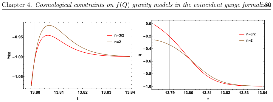
The $\alpha Q+\beta Q^n$ class gives a single geometric dark-energy fluid that interpolates between quintessence ($n\ge1$), phantom ($n\le-1$), and $\Lambda$CDM ($n=0$) behavior, meaning one family of actions covers the main dark-energy phenomenologies.
The non-coincident connection with $\gamma(t)=-a^{-1}\dot H$ yields Friedmann equations that are not equivalent to $f(T)$ gravity, so parameter constraints obtained in this formalism are new information rather than a re-derivation of known results.
The explicit caveat that these solutions cannot describe the early Universe implies the models are late-time effective descriptions only, not full cosmic histories.

Reading between the lines

Editorial extensions of the paper, not claims the author makes directly.

Editorial inference: because the fitted forms for $\xi$, $f(Q)$, and $H(z)$ are chosen rather than derived, the numerical constraints, such as $H_0=68\pm0.094$ km/s/Mpc and $z_t=0.857\pm0.011$, should be read as attached to those ansatze; a different equally reasonable choice could shift the best-fit values by more than the quoted $1\sigma$ errors.
Editorial inference: the same parameterization machinery could be extended to early-Universe probes such as CMB acoustic-scale distances or primordial nucleosynthesis abundances; the thesis's own admission that the solutions fail at early times suggests such an extension would be the immediate stress test.
Editorial inference: the connection function $\gamma(t)=-a^{-1}\dot H$ is itself an ansatz; exploring other non-constant $\gamma(t)$ choices would show whether the claimed late-time fits are robust features of non-coincident $f(Q)$ gravity or artifacts of this particular gauge connection.

Share X Bluesky LinkedIn Reddit HN

Editorial analysis

A structured set of objections, weighed in public.

Desk editor's note, referee report, and a circularity audit.

Desk Editor's Note

read the letter

The honest summary: this is a PhD thesis that assembles the author's own published papers into one document. The core results—viscous f(Q) solutions, the αQ+βQ^n constraints, the non-coincident Hubble parameterization—are not new relative to those papers. What the thesis does well is present them coherently, with the derivations mostly consistent and the analytical solutions checked against data. It also states plainly that these models do not describe the early Universe, which is a real limitation acknowledged up front. For someone entering f(Q) cosmology, this is a serviceable starting point.

The soft spot that matters is in Sec. 2.5.2. The Pantheon chi-square marginalization formula defines B identically to A—both have the squared residual. The standard marginalization over the additive nuisance μ0 requires B = Σ [μth(μ0=0) − μobs]/σ², without the square. As written, the formula is self-contradictory. If that formula was actually used in the MCMC, the quoted best-fit parameters and contours in Chapter 2, and by extension the abstract's claim about describing cosmic acceleration, are not reproducible. This is a load-bearing statistical error, not a typo you can wave off. The underlying published paper (Phys. Dark Univ. 32, 100820) may have had it right, but this thesis as posted does not.

Other soft spots are lighter. Chapters 4 and 5 fix parameters from the same data they then compare against, so this is fitting rather than prediction—common in this literature, and the thesis does not aggressively oversell it. The viscosity ansatz and the connection function γ(t) = −a⁻¹Ḣ are hand-picked, with no derivation from microphysics or the f(Q) action. That limits how strongly you can interpret the 'predictions.' Minor: the evolutionary profiles in later chapters lack uncertainty bands.

Bottom line: the central idea that bulk viscosity in f(Q) gravity can mimic late-time acceleration is plausible and consistent with earlier work, but the statistical validity of the headline fits is compromised as written. The thesis deserves a serious referee only if the chi-square issue is fixed first. For my own work, I would cite the original journal articles, not this arXiv posting—though I might point a starting student to it for the broad overview.

Referee Report

4 major / 4 minor

Summary. The thesis (arXiv:2502.10466) develops cosmological models in modified symmetric teleparallel gravity. It derives exact Hubble solutions for linear and power-law f(Q) gravity with bulk viscous fluids, fits the resulting models to Hubble, Pantheon, BAO, and Pantheon+SH0ES data, and uses the fits to claim a late-time deceleration-to-acceleration transition and quintessence, phantom, and Lambda-CDM-like effective behavior. It also presents a non-coincident connection framework with a parameterized Hubble function, applies energy conditions and sound-speed stability tests to several STEGR corrections, and closes with a covariant formulation and phase-space analysis of f(Q,T) gravity. The abstract explicitly concedes that the bulk-viscous solutions cannot describe the early Universe.

Significance. If the statistical results can be made reproducible, the thesis would be a useful collection of exact f(Q) cosmologies: the field-equation manipulations and analytical integrations are largely self-consistent, the non-coincident connection calculations in Chapter 5 go beyond the usual coincident-gauge treatment, and the f(Q,T) covariant formulation in Chapter 6 is a valuable reference point. The manuscript also has the merit of being explicit about its main limitation, namely that the bulk-viscous solutions fail in the early Universe. However, the central late-time claims currently rest on a printed chi-square marginalization that is algebraically wrong, and the Chapter 4 conclusions are obtained by fixing model parameters to the very observables the model is then said to reproduce. These issues must be addressed before the data-driven conclusions can be accepted.

major comments (4)

[Sec. 2.5.2, Eq. (2.28) and the following display] The quantities A and B are printed identically: B is defined as the same sum of squared residuals as A. For a Gaussian marginalization over an additive nuisance mu0, the correct profile chi-square is A - B^2/C with B = sum_i [mu_th(mu0=0,z_i,theta)-mu_obs(z_i)]/sigma_i^2, i.e., the linear residual, not the squared residual. As written, the 'marginalized' chi-square is A - A^2/C, which is not the likelihood marginalized over mu0 and can bias the parameter estimates. The Pantheon best-fit values (alpha=-1.33, xi0=0.10, xi1=1.81, xi2=2.08), the contours in Figs. 2.7 and 2.10, and the statefinder statements based on those parameters are therefore not reproducible from the text. This must be corrected and the fits rerun before the Chapter 2 claim of describing late-time acceleration can be evaluated.
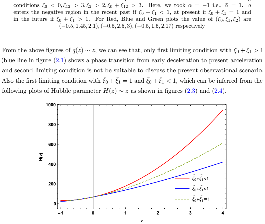
[Sec. 4.4-4.6, Eqs. (4.22)-(4.23)] The parameters alpha and beta are fixed by solving Eqs. (4.22) and (4.23) using the observed values H0=67.9 km/s/Mpc, q0=-0.55, and Omega0=0.303, and the subsequent sections then show that the model reproduces quintessence, phantom, or Lambda-CDM-like behavior for different choices of n. This is a demonstration that the ansatz can be tuned to the target observables, not an independent observational validation. No MCMC fit with propagated uncertainties is presented for the n>=1 and n<=-1 cases. The text should either reframe Sections 4.4-4.6 as existence/tuning examples or perform a genuine data fit and report the resulting parameter uncertainties.
[Sec. 5.2, Eq. (5.12)] The Hubble parameterization H(z)=H0(z+1)^n + beta[1-(z+1)^n] and the connection function gamma(t)=-a^{-1}Hdot are assumed without derivation from the f(Q) action or from microphysics. All subsequent constraints on Models I-V via energy conditions and sound speed are therefore conditional on these choices. The text should state this limitation explicitly and, ideally, test robustness by considering alternative parameterizations of H(z) or alternative non-constant gamma(t), since a different ansatz will in general change the fitted parameters, the transition redshift, and the derived energy-condition profiles.
[Sec. 3.3.3, Eq. (3.13)] The Pantheon likelihood in Eq. (3.13) uses only the diagonal errors sigma(zk) and does not show the standard marginalization over the absolute magnitude nuisance parameter. The Pantheon release includes a full covariance matrix with systematic uncertainties, and the usual analysis either uses that covariance or explicitly marginalizes over M. As printed, the reported 1-sigma contours in Fig. 3.4 are likely optimistic. Please clarify the treatment of systematics and either use the full covariance or state and justify the diagonal approximation.

minor comments (4)

[Sec. 5.3.3] The statement that DeltaBIC=6.869 constitutes 'strong evidence' is inconsistent with the thresholds given in the same paragraph, where 2-6 is called moderate and >10 is called no support. Please correct the interpretation or the threshold convention.
[Figs. 3.5-3.12 and 5.2] The evolutionary profiles of H, q, rho, p, omega, and the energy conditions are plotted only as central curves. Adding 1-sigma and 2-sigma bands propagated from the MCMC chains would make the fits quantitatively comparable and would strengthen the claims about the deceleration-to-acceleration transition.
[Throughout] Several typographical errors should be corrected in a revised version: 'Reimannian' for 'Riemannian', 'charateristics' for 'characteristics', 'Ries' for 'Riess', and the spacing in 'T ee-How' and 'W eak'.
[Abstract and Sec. 7.1] The abstract's admission that the bulk-viscous solutions cannot describe the early phases is an important scope limitation and should be restated in the concluding chapter rather than only in the abstract, so that readers do not over-interpret the late-time fits as a complete cosmological model.

Circularity Check

2 steps flagged · score 6.0 of 10

Partial circularity: the late-time acceleration 'prediction' is calibrated or built into the chosen ansätze (Eqs. 4.22-4.23 and Eq. 5.12), while most of the derivation itself is self-contained.

fitted input called prediction [Chapter 4, Sec. 4.3 and Sec. 4.8, Eqs. (4.22)-(4.23) and (4.12).]
"Our aim is to estimate the value of parameters of a given f (Q) model that would be in agreement with the recently observed values of the cosmographic parameters. By using equations (4.20) and (4.21), we obtain the values of model parameters α and β in terms of present value cosmographic parameters and the power of non-metricity term n, as, α = ... (4.22) and β = ... (4.23) ... Now, we solve the differential equation (4.12) by the numerical algorithm with initial conditions as H0 = 67.9 km/s/Mpc, q0 = −0.55, Ω0 = 0.303 ..."

The parameters α and β are algebraically solved from the target values q0, H0, Ω0. The chapter then uses this calibrated solution to report quintessence, phantom, and ΛCDM-like behaviors as the model's dark-energy scenario. The present acceleration q0 is thus an input used to determine the model, not an output predicted from the f(Q) action; the classification by n follows from the chosen ansatz f(Q)=αQ+βQ^n after forcing the cosmographic parameters.
self definitional [Chapter 5, Secs. 5.2 and 5.3.4, Eq. (5.12).]
"In addition, we propose a new parameterization of the Hubble function that can consistently depicts the present deceleration parameter value, transition redshift, and the late time de-Sitter limit. ... H(z) = H0(z + 1)^n + β [1 − (z + 1)^n] . (5.12) ... From figure (5.2) it is evident that the proposed function predicts the de-Sitter type accelerated expansion phase at the late times via a transition epoch from the decelerated epoch to accelerated epoch in the recent past with the transition redshift zt = 0.857 ± 0.011."

The Hubble ansatz was chosen specifically to contain a present deceleration value, a transition redshift, and a de Sitter limit. For any fitted n>0, Eq. (5.12) gives q→−1 at z→−1 and q→n−1 at z→∞, so a deceleration-to-acceleration transition is guaranteed by the functional form, not by the data. Calling this a 'prediction' restates the design specification; only the fitted numbers (H0,β,n) and zt=0.857 are data-dependent.

full rationale

Most of the mechanical derivation is self-contained and not circular: the f(Q) field equations are obtained from the action in Chapter 1, the linear and power-law viscous solutions in Chapters 2-3 follow by integration from stated bulk-viscosity and f(Q) assumptions, and the parameter values are obtained by emcee fits to standard external datasets (CC, Pantheon, BAO, Pantheon+SH0ES). I find no load-bearing self-citation or imported uniqueness theorem; the cited prior framework for the non-coincident connection in Chapter 5 is an explicit ansatz, not a uniqueness claim. The circularity is partial, in two places where the paper presents calibrated or in-built properties as predictions. First, Chapter 4 solves α, β from the target q0, H0, Ω0 (Eqs. 4.22-4.23), so the reported late-time acceleration is an input. Second, Chapter 5 defines an H(z) family whose qualitative transition and de Sitter limit are guaranteed for fitted n>0, and then reports that the function 'predicts' that transition. The quantitative fits are still informative, and the n=0 case is honestly labeled as mimicking ΛCDM, so the thesis is not a pure tautology. Separately, the printed Pantheon marginalization in Sec. 2.5.2 defines B identically to A; that is a statistical error that would bias the quoted Pantheon contours, but it is a computational issue rather than a circularity. The abstract's limitation that these solutions 'cannot describe the early phases of the Universe' is an honest scope statement and does not affect the circularity verdict.

Assumptions & free parameters 6 free parameters · 5 assumptions · 0 invented entities

The central models rest on the FLRW symmetry assumption, the perfect-fluid bulk-viscous stress-energy, and several hand-chosen functional forms (viscosity law, connection function, Hubble parameterization). Many free parameters are fitted to the same datasets used to validate the models.

free parameters (6)

alpha (f(Q) = alpha Q) = alpha = -1.03 (Hubble), -1.33 (Pantheon), -1.06 (Hubble+BAO), -1.65 (Pantheon+BAO)
Scales the non-metricity action in Chapter 2; fixed by fitting H(z) and Pantheon data.
xi0, xi1, xi2 (bulk viscosity coefficients) = xi0=1.54, xi1=0.08, xi2=0.66 (Hubble); xi0=0.10, xi1=1.81, xi2=2.08 (Pantheon)
Dimensionless coefficients in the viscosity ansatz Eq. (2.6); constrained by the same data.
alpha, n (f(Q) = alpha Q^n) = alpha=-0.0166, n=0.974 (Hubble); alpha=-0.0125, n=0.996 (BAO); alpha=-0.00999, n=1.001 (Pantheon)
Power-law f(Q) model in Chapter 3; fitted to the datasets.
zeta (bulk viscosity coefficient) = zeta=0.65 (Hubble), 0.66 (BAO), 0.67 (Pantheon)
Constant bulk viscosity in Chapter 3; fitted.
beta, n (f(Q) = alpha Q + beta Q^n) = beta=-26.01, n=0 for the alpha Q + beta case; n chosen as 3/2, 2, -1, -2 by hand
Chapter 4; for the exact solution n=0, beta is fitted; for other n, alpha and beta are derived from q0, H0, Omega0.
H0, beta, n (Hubble parameterization) = H0=68 +/- 0.094, beta=42, n=1.6
Chapter 5; fitted to CC+Pantheon+SH0ES+BAO.

assumptions (5)

domain assumption Spatially flat FLRW metric
All chapters use the flat FLRW line element (Eqs. 2.1, 5.1); deviations from flatness are not considered.
domain assumption Bulk viscous perfect fluid stress-energy
Matter is modeled as non-relativistic dust with bulk viscosity, with p=0 and viscosity law Eq. (2.6) or constant zeta; this is not derived.
ad hoc to paper Connection function gamma(t) = -a^-1 Hdot
Chapter 5 assumes this non-vanishing connection component to generate equations distinct from f(T); no derivation from the action is given.
ad hoc to paper Hubble parameterization H(z) = H0(z+1)^n + beta [1 - (z+1)^n]
Proposed in Sec. 5.2 as a three-parameter fit; all Chapter 5 constraints depend on this un-derived form.
standard math Standard statistical inference tools
Chi-square minimization, MCMC/emcee, AIC/BIC are used as standard practice; their validity is assumed.

how reviews work

0 comments

Cite this review

Pith. "Pith review of Accelerating Expansion of the Universe in Modified Symmetric Teleparallel Gravity." pith.science (2026). https://pith.science/paper/4CFTIELU

@misc{pith2026250210466,
  author       = {Pith},
  title        = {Pith review of: Accelerating Expansion of the Universe in Modified Symmetric Teleparallel Gravity},
  year         = {2026},
  howpublished = {\url{https://pith.science/paper/4CFTIELU}},
  note         = {Machine review of arXiv:2502.10466}
}

read the original abstract

In the last century, theoretical and experimental developments have established the General Relativity theory as the most successful theory for describing the gravitational phenomenon. On the other hand, in the last two decades, multiple observational probes have strongly favored the discovery of the acceleration of cosmic expansion. The observational enhancement and development in precision cosmology indicate a requirement to go beyond General Relativity and to search for an alternate description that can resolve the persistent issues. In Chapter 1, we highlight some important elements of observational cosmology. In Chapters 2 and 3, we investigate the f(Q) gravity in the presence of viscosity in the cosmic fluid. In Chapters 4 and 5, we explore the constraints on the various classes of non-linear f(Q) gravity models in both coincident and non-coincident formalism, respectively. In Chapter 6, we present a covariant formulation and energy balance equation for the f(Q,T) gravity, which is an extension of f(Q) gravity. Finally, in Chapter 7, we briefly summarize the outcomes of the present thesis and the future scope.

Figures

Figures reproduced from arXiv: 2502.10466 by the authors.

**Figure 1.1.** Flow chart representing the steps to construct a cosmological model. 1.5.2 χ 2 minimization Consider a function fmodel(x, θ) in the independent variable x and the set of free parameters θ. If the set {fk,obs(xk,obs)} n k=1 represents n independent observation along with the standard deviation σk,obs, then we define the χ 2 as follows [58], χ 2 (θ) = Xn k=1 (fmodel(xk,obs, θ) − fk,obs) 2 σ 2 k,obs . (1.108) Moreover,… view at source ↗

**Figure 2.1.** Variation of the deceleration parameter with redshift z for the first limiting conditions ¯ξ0 > 0, ¯ξ12 < 3, ¯ξ2 < 2, ¯ξ0 + ¯ξ12 < 3. Here, we took α = −1 i.e., α¯ = 1. q enters the negative region in the recent past if ¯ξ0 + ¯ξ1 > 1, at present if ¯ξ0 + ¯ξ1 = 1 and in the future if ¯ξ0 + ¯ξ1 < 1. For Red, Blue and Green plots the value of (¯ξ0, ¯ξ1, ¯ξ2) are (0.9, 0.01, 1),(0.45, 0.65, 1),(0.65, 0.35, 1) respective… view at source ↗

**Figure 2.2.** Variation of the deceleration parameter with redshift z for the second limiting conditions ¯ξ0 < 0, ¯ξ12 > 3, ¯ξ2 > 2, ¯ξ0 + ¯ξ12 > 3. Here, we took α = −1 i.e., α¯ = 1. q enters the negative region in the recent past if ¯ξ0 + ¯ξ1 < 1, at present if ¯ξ0 + ¯ξ1 = 1 and in the future if ¯ξ0 + ¯ξ1 > 1. For Red, Blue and Green plots the value of (¯ξ0, ¯ξ1, ¯ξ2) are (−0.5, 1.45, 2.1),(−0.5, 2.5, 3),(−0.5, 1.5, 2.17) respe… view at source ↗

Figures from the paper (55 more)

**Figure 2.3.** Figure 2.3: Variation of the Hubble parameter with redshift z for the first limiting conditions ¯ξ0 > 0, ¯ξ12 < 3, ¯ξ2 < 2, ¯ξ0 + ¯ξ12 < 3. Here we took α = −1 i.e., α¯ = 1. For Red, Blue and Green plots the value of (¯ξ0, ¯ξ1, ¯ξ2) are (0.9, 0.01, 1),(0.45, 0.65, 1),(0.65, 0.35…

**Figure 2.4.** Figure 2.4: Variation of the Hubble parameter with redshift z for the second limiting conditions ¯ξ0 < 0, ¯ξ12 > 3, ¯ξ2 > 2, ¯ξ0 + ¯ξ12 > 3. Here we took α = −1 i.e., α¯ = 1. For Red, Blue and Green plots the value of (¯ξ0, ¯ξ1, ¯ξ2) are (−0.5, 1.45, 2.1),(−0.5, 2.5, 3),(−0.5, 1…

**Figure 2.5.** Figure 2.5: The plot shows the 2-d contour plots of the model parameters with 1 − σ and 2 − σ errors and also shows the best fit values of the model parameters α, ξ0, ξ1 and ξ2 obtained from the 57 points of Hubble datasets [PITH_FULL_IMAGE:figures/full_fig_p060_2_5.png]

**Figure 2.6.** Figure 2.6: The plot shows the plot of Hubble function H(z) vs. redshift z for our model shown in red line which shows nice fit to the 57 points of the Hubble datasets shown in dots with it’s error bars and also compared to the ΛCDM model shown in black solid line with Ωm0 = 0.3…

**Figure 2.7.** Figure 2.7: The plot shows the best fit values of the model parameters α, ξ0, ξ1 and ξ2 obtained w.r.t to the 1048 points of Pantheon datasets at 1 − σ and 2 − σ confidence level [PITH_FULL_IMAGE:figures/full_fig_p063_2_7.png]

**Figure 2.8.** Figure 2.8: The plot shows the plot of distance modulus µ(z) vs. redshift z for our model shown in red line which shows nice fit to the 1048 points of the Pantheon datasets shown in dots with it’s error bars. 2.5.3 BAO datasets In the study of the early Universe baryons, photons…

**Figure 2.9.** Figure 2.9: The plot shows the 2-d contour plots of the model parameters with 1 − σ and 2 − σ errors and also shows the best fit values of the model parameters α, ξ0, ξ1 and ξ2 obtained from the 57 points of Hubble datasets together with six points of BAO datasets [PITH_FULL_IM…

**Figure 2.10.** Figure 2.10: The plot shows the best fit values of the model parameters α, ξ0, ξ1 and ξ2 obtained w.r.t to the 1048 points of Pantheon datasets together with six points of BAO datasets at 1 − σ and 2 − σ confidence level. 2.6 Statefinder diagnostic It is well-known that the dece…

**Figure 2.11.** Figure 2.11: The evolution trajectories of the given model in s − r plane for the free parameter values obtained by the Hubble and Pantheon datasets [PITH_FULL_IMAGE:figures/full_fig_p068_2_11.png]

**Figure 2.12.** Figure 2.12: The evolution trajectories of the given model in q − r plane for the free parameter values obtained by the Hubble and Pantheon datasets. The fixed point (s, r) = (0, 1) in the s − r diagram (2.11) shows the spatially flat ΛCDM model and (q, r) = (−1, 1) shows the de…

**Figure 2.13.** Figure 2.13: The evolution trajectories of the given model in s − r plane for the free parameter values obtained by the Hubble and Pantheon datasets together with BAO datasets. Hubble+BAO Pantheon+BAO dS ΛCDM Quintessence -1.0 -0.5 0.0 0.5 1.0 1.5 2.0 0.0 0.5 1.0 1.5 2.0 2.5 3.0…

**Figure 2.14.** Figure 2.14: The evolution trajectories of the given model in q − r plane for the free parameter values obtained by the Hubble and Pantheon datasets together with BAO datasets [PITH_FULL_IMAGE:figures/full_fig_p070_2_14.png]

**Figure 3.1.** Figure 3.1: The 1−σ and 2−σ likelihood contours for the model parameters using the Hubble datasets [PITH_FULL_IMAGE:figures/full_fig_p077_3_1.png]

**Figure 3.2.** Figure 3.2: The error bar plot of H versus z for the considered f(Q) model. The solid red line is the curve for f(Q) model whereas the black dotted line represents the ΛCDM model. The blue dots depict the 31 points of the Hubble data. The obtained suitable values of the free par…

**Figure 3.3.** Figure 3.3: The 1 − σ and 2 − σ likelihood contours for the model parameters using the BAO datasets. 3.3.3 Pantheon datasets Scolnic et al. [19] put together the Pantheon samples consisting of 1048 type Ia supernovae in the redshift range 0.01 < z < 2.3. The PanSTARSS1 Medium De…

**Figure 3.4.** Figure 3.4: The 1 − σ and 2 − σ likelihood contours for the model parameters using the Pantheon datasets. 3.3.4 Cosmological parameters The evolution trajectories of the Hubble function, deceleration parameter, energy density, pressure with bulk viscosity and the effective EoS p…

**Figure 3.5.** Figure 3.5: Profile of the Hubble parameter for the given model with the parameter values estimated by the Hubble, BAO and the Pantheon data point sets. Hubble BAO Pantheon 0 2 4 6 8 -1.0 -0.5 0.0 0.5 1.0 z q [PITH_FULL_IMAGE:figures/full_fig_p082_3_5.png]

**Figure 3.6.** Figure 3.6: Profile of the deceleration parameter for the given model with the parameter values estimated by the Hubble, BAO and the Pantheon data point sets. Hubble BAO Pantheon 0 2 4 6 8 0 20 000 40 000 60 000 80 000 z ρ [PITH_FULL_IMAGE:figures/full_fig_p082_3_6.png]

**Figure 3.7.** Figure 3.7: Profile of the density parameter for the given model with the parameter values estimated by the Hubble, BAO and the Pantheon data point sets [PITH_FULL_IMAGE:figures/full_fig_p082_3_7.png]

**Figure 3.8.** Figure 3.8: Profile of the pressure for the given model with the parameter values estimated by the Hubble, BAO and the Pantheon data point sets. Hubble BAO Pantheon 0 2 4 6 8 -1.0 -0.8 -0.6 -0.4 -0.2 0.0 0.2 0.4 z ωeff [PITH_FULL_IMAGE:figures/full_fig_p083_3_8.png]

**Figure 3.9.** Figure 3.9: Profile of the EoS parameter for the given model with the parameter values estimated by the Hubble, BAO and the Pantheon data point sets. From figure (3.6), it is clear that the deceleration parameter shows the transition from a decelerated (q > 0) to an accelerated …

**Figure 3.10.** Figure 3.10: Profile of the null energy condition for the given model with the parameter values estimated by the Hubble, BAO and the Pantheon data point sets [PITH_FULL_IMAGE:figures/full_fig_p084_3_10.png]

**Figure 3.11.** Figure 3.11: Profile of the dominant energy condition for the given model with the parameter values estimated by the Hubble, BAO and the Pantheon data point sets. Hubble BAO Pantheon Hubble BAO Pantheon -1.0 -0.5 0.0 0.5 1.0 -100 0 100 200 300 z SEC 0 2 4 6 8 0 50 000 100 000 15…

**Figure 3.12.** Figure 3.12: Profile of the strong energy condition for the given model with the parameter values estimated by the Hubble, BAO and the Pantheon data point sets. 3.5 Statefinder analysis For different values of the statefinder pair (r, s), it represents the following dark energy …

**Figure 3.13.** Figure 3.13: Plot of the trajectories in the r − s plane for the given cosmological model with the parameter values estimated by the Hubble, BAO and the Pantheon datasets. Hubble BAO Pantheon dS ΛCDM Quintessence -1.0 -0.8 -0.6 -0.4 -0.2 0.0 0.2 0.4 0.4 0.6 0.8 1.0 1.2 1.4 1.6 q…

**Figure 3.14.** Figure 3.14: Plot of the trajectories in the q − r plane for the given cosmological model with the parameter values estimated by the Hubble, BAO, and the Pantheon datasets. Figures (3.13) and (3.14) show that our bulk viscous model lies in the quintessence region. Also, [PITH_F…

**Figure 4.1.** Figure 4.1: Profile of the dimensionless density parameter and the energy density for the dark energy component vs cosmic time t [PITH_FULL_IMAGE:figures/full_fig_p094_4_1.png]

**Figure 4.2.** Figure 4.2: Profile of the EoS parameter for the dark energy component and the deceleration parameter vs cosmic time t. n=3/2 n=2 13.795 13.800 13.805 13.810 13.815 13.820 0 5000 10 000 15 000 20 000 t ρ m n=3/2 n=2 13.79 13.80 13.81 13.82 13.83 13.84 -1.0 -0.9 -0.8 -0.7 -0.6 -0…

**Figure 4.3.** Figure 4.3: Profile of the matter-energy density and the effective EoS parameter vs cosmic time t. From figures (4.1) and (4.3) (left panel), we found that the both matter-energy density and dark energy density of the Universe decrease with cosmic time and matter energy density …

**Figure 4.4.** Figure 4.4: Profile of the effective energy density and the NEC vs cosmic time t. n=3/2 n=2 13.795 13.800 13.805 13.810 13.815 13.820 20 000 30 000 40 000 50 000 t DEC n=3/2 n=2 13.795 13.800 13.805 13.810 13.815 13.820 -18 000 -17 000 -16 000 -15 000 t SEC [PITH_FULL_IMAGE:fig…

**Figure 4.5.** Figure 4.5: Profile of the DEC and the SEC vs cosmic time t. From figure (4.4) (left panel) it is clear that the effective energy density show positive behavior. Moreover from figures (4.4) (right panel) and (4.5) we found that NEC, WEC, and DEC are satisfied while the SEC is vi…

**Figure 4.6.** Figure 4.6: Profile of the dimensionless density parameter and the energy density for the dark energy component vs cosmic time t. n=-1 n=-2 13.795 13.800 13.805 13.810 -1.0 -0.8 -0.6 -0.4 -0.2 0.0 t wDE n=-1 n=-2 13.796 13.798 13.800 13.802 13.804 -1.0 -0.5 0.0 0.5 t q [PITH_FU…

**Figure 4.7.** Figure 4.7: Profile of the EoS parameter for the dark energy component and the deceleration parameter vs cosmic time t. n=-1 n=-2 13.796 13.797 13.798 13.799 13.800 13.801 13.802 0 10 000 20 000 30 000 40 000 50 000 60 000 t ρ m n=-1 n=-2 13.795 13.800 13.805 13.810 13.815 13.82…

**Figure 4.8.** Figure 4.8: Profile of the matter-energy density and the effective EoS parameter vs cosmic time t. From figures (4.6) and (4.8) (left panel), we found that the matter-energy density of the Universe decrease with cosmic time while dark energy density increases with time. Moreover…

**Figure 4.9.** Figure 4.9: Profile of the effective energy density and the NEC vs cosmic time t. n=-1 n=-2 13.800 13.805 13.810 13.815 13.820 20 000 25 000 30 000 t DEC n=-1 n=-2 13.800 13.805 13.810 13.815 13.820 -22 000 -20 000 -18 000 -16 000 -14 000 -12 000 -10 000 -8000 t SEC [PITH_FULL_…

**Figure 4.10.** Figure 4.10: Profile of the DEC and the SEC vs cosmic time t. From figure (4.9) (left panel) it is clear that the effective energy density show positive behavior. Moreover from figures (4.9) (right panel) and (4.10) we found that NEC and SEC are violated. By the definition of en…

**Figure 4.11.** Figure 4.11: Profile of the dimensionless density parameter for the dark energy component, the effective EoS parameter, and the deceleration parameter vs cosmic time t. In this case, we have obtained constant negative pressure with dark energy EoS parameter follows the ΛCDM EoS.…

**Figure 4.12.** Figure 4.12: The 1 − σ and 2 − σ likelihood contours for the model parameters using the combination CC+BAO+Pantheon datasets [PITH_FULL_IMAGE:figures/full_fig_p100_4_12.png]

**Figure 4.13.** Figure 4.13: Profile of the density of the dark energy component and the deceleration parameter vs redshift z . -1 0 1 2 3 4 -1.0 -0.8 -0.6 -0.4 -0.2 0.0 z wDE -1 0 1 2 3 4 -1.0 -0.8 -0.6 -0.4 -0.2 0.0 z weff [PITH_FULL_IMAGE:figures/full_fig_p101_4_13.png]

**Figure 4.14.** Figure 4.14: Profile of the EoS parameter for the dark energy component and the effective EoS parameter vs redshift z . Form figure (4.13) (left panel) it is clear that the energy density of the dark energy component of the Universe decreases with cosmic time and it falls off to…

**Figure 5.1.** Figure 5.1: The contour plot for the free parameter space (H0, β, n) corresponding to the given Hubble function within the 1σ − 3σ confidence interval using CC+Pantheon+SH0ES+BAO samples. We obtained the free parameter constraints as H0 = 68 ± 0.094 km/s/M pc, β = 42+0.04 −0.041…

**Figure 5.2.** Figure 5.2: Profile of the jerk, snap, and the deceleration parameter vs redshift. It is well known that the cosmographic parameters can be obtained as the coefficient of the Taylor series expansion of the scale factor with the present time as the center. The coefficient of term…

**Figure 5.3.** Figure 5.3: Profile of the SEC and the NEC vs redshift, corresponding to the Model-I with varying α and fixed η = 1 [PITH_FULL_IMAGE:figures/full_fig_p112_5_3.png]

**Figure 5.4.** Figure 5.4: Profile of the SEC and the NEC vs redshift, corresponding to the Model-I with varying η and fixed α = 1. Model-I: The Model-I is an exponential correction to the STEGR case. From figures (5.3) and (5.4), it is clear that, in the entire range of redshift, the NEC is s…

**Figure 5.5.** Figure 5.5: Profile of the SEC and the NEC vs redshift, corresponding to the Model-II with varying α and fixed η = 1 [PITH_FULL_IMAGE:figures/full_fig_p113_5_5.png]

**Figure 5.6.** Figure 5.6: Profile of the SEC and the NEC vs redshift, corresponding to the Model-II with varying η and fixed α = −1. Model-II: The Model-II is an logarithmic correction to the STEGR case. From figures (5.5) and (5.6), it is clear that, in the entire range of redshift, the NEC …

**Figure 5.7.** Figure 5.7: Profile of the SEC and the NEC vs redshift, corresponding to the Model-III with varying α and fixed η = 1. Model-III: The Model-III is a power-law correction to the STEGR case. From figure (5.7), it is evident that, in the entire range of redshift, the NEC is satisfi…

**Figure 5.8.** Figure 5.8: Profile of the SEC and the NEC vs redshift, corresponding to the Model-IV with varying η and fixed α = −1. Model-IV: The Model-IV is a negative power-law correction to the STEGR case. A negative power correction to the STEGR case provides a correction to the late-tim…

**Figure 5.9.** Figure 5.9: Profile of the SEC and the NEC vs redshift, corresponding to the Model-V with varying η and fixed α = 2. Model-V: The Model-V is a positive power-law correction to the STEGR case. A positive power correction to the STEGR case provides a correction to the early epochs…

**Figure 5.10.** Figure 5.10: Profile of the sound speed parameter vs z (redshift) for the Model-I corresponding to the case varying η with α = 1 (left panel) and the varying α with η = 1 (right panel). From figure (5.10), one can observe that the sound speed parameter for the Model-I lies betwe…

**Figure 5.11.** Figure 5.11: Profile of the sound speed parameter vs z (redshift) for the Model-II corresponding to the case varying η with α = −1 (left panel) and the varying α with η = 1 (right panel). From figure (5.11), it is evident that the sound speed parameter for the Model-II lies betw…

**Figure 5.12.** Figure 5.12: Profile of the sound speed parameter vs z (redshift) for the Model-III with varying α and η = 1 (left panel), Model-IV with varying η and α = −1 (middle panel), and the Model-V with varying η and α = 2 (right panel). From figure (5.12) (left panel), we find that the…

**Figure 6.1.** Figure 6.1: Phase plots corresponding to the case β = 0 with κ = 1. For the case β = 0, the obtained critical points are P(1,1) and Q(1,0) with corresponding eigenvalues 0, 3 2 and 0, − 3 2 respectively. From figure (6.1), it is evident that the trajectories are emerging from th…

**Figure 6.2.** Figure 6.2: Phase plot corresponding to the model f(Q, T) = αQ + βT2 with κ = 1. From figure (6.2), it is evident that the critical points A(0,0) and B(1,1) are saddle points, whereas the critical point C(1,0) indicates a stable matter dominated epoch. The critical point D(0,1) …

**Figure 6.3.** Figure 6.3: Phase plots corresponding to the case β = 0 with κ = 1 and ¯α = 1. For the case β = 0 with κ = 1 and α¯ = 1, the obtained critical points are A(1,0), B(1,1), and C(1,0.5). From Table (6.3) and figure (6.3), it is evident that the critical points A(1,0) and C(1,0.5) w…

Discussion (0). Continue with ORCID to comment.

Reference graph

Works this paper leans on

263 extracted references · 76 canonical work pages

[1]

Hubble, Proc

E. Hubble, Proc. N. A. S. 15, 168 (1929)

1929
[2]

Hubble, M

E. Hubble, M. L. Humason, Astrophys. J. 74, 43 (1931)

1931
[3]

Aghanim, et al., Astron

Planck Collaboration, N. Aghanim, et al., Astron. Astrophys. 641, A6 (2020)

2020
[4]

Aiola et al., J

S. Aiola et al., J. Cosmol. Astropart. Phys. 12, 047 (2020)

2020
[5]

Dutcher et al., Phys

D. Dutcher et al., Phys. Rev. D 104, 022003 (2021)

2021
[6]

Alam et al., Phys

S. Alam et al., Phys. Rev. D 103, 083533 (2021)

2021
[7]

A. G. Riess et al., Astrophys. J. 876, 85 (2019)

2019
[8]

A. G. Riess et al., Astrophys. J. Lett. 908, L6 (2021)

2021

Show all 263 references

[9]

Hillebrandt, J

W. Hillebrandt, J. C. Niemeyer, Ann. Rev. Astron. Astrophys. 38, 191 (2000)

2000
[10]

A. G. Riess et al., Astron. J. 116, 1009 (1998)

1998
[11]

Perlmutter et al., Astrophys

S. Perlmutter et al., Astrophys. J. 517, 565 (1999)

1999
[12]

R. A. Scalzo et al., Astrophys. J. 713, 1073 (2009)

2009
[13]

J. A. Holtzman et al., Astron. J. 136, 2306 (2008)

2008
[14]

Leaman et al., Mon

J. Leaman et al., Mon. Not. R. Astron. Soc. 412, 1419 (2011)

2011
[15]

Astier et al., Astron

P. Astier et al., Astron. Astrophys. 447, 31 (2006)

2006
[16]

Kowalski et al., Astrophys

M. Kowalski et al., Astrophys. J. 686, 749 (2008)

2008
[17]

Amanullah et al., Astrophys

R. Amanullah et al., Astrophys. J. 716, 712 (2010)

2010
[18]

Suzuki et al., Astrophys

N. Suzuki et al., Astrophys. J. 746, 85 (2012)

2012
[19]

D. M. Scolnic et al., Astrophys. J. 859, 101 (2018)

2018
[20]

Brout et al., Astrophys

D. Brout et al., Astrophys. J. 938, 110 (2022). 123 References 124

2022
[21]

Lemaitre, Mon

G. Lemaitre, Mon. Not. R. Astron. Soc. 91, 490 (1931)

1931
[22]

A. A. Penzias, R. W. Wilson, Astrophys. J. 142, 419 (1965)

1965
[23]

R. H. Dicke et al., Astrophys. J. 412, 414 (1965)

1965
[24]

D. J. Fixsen et al., Astrophys. J. 473, 576 (1996)

1996
[25]

A. A. Michelson, E. Morley, Am. J. Sci. 34, 333-345 (1887)
[26]

Einstein, Ann

A. Einstein, Ann. Phys. 17, 891-921 (1905)

1905
[27]

J. B. Hartle, “Gravity” ( Pearson) (2003)

2003
[28]

Spacetime and Geometry: An Introduction to GR

S. Carroll, “Spacetime and Geometry: An Introduction to GR” ( Addison Wesley, Boston ) (2004)

2004
[29]

Einstein, Ann

A. Einstein, Ann. Phys. 354, 769-822 (1916)

1916
[30]

H. P. Robertson, Astrophys. J. 82, 284 (1935)

1935
[31]

A. G. Walker, Proc. Lon. Math. Soc. 42, 90127 (1937)

1937
[32]

Einstein, Sitzber

A. Einstein, Sitzber. Preuss. Akad. Wiss. 142, 87 (1917)

1917
[33]

Einstein, Sitzber

A. Einstein, Sitzber. Preuss. Akad. Wiss. 235, 37 (1931)

1931
[34]

Y. B. Zel ´dovich, JETP Lett. 6, 316 (1967)

1967
[35]

Weinberg, Phys

S. Weinberg, Phys. Rev. Lett. 59, 2607 (1987)

1987
[36]

Abdalla et al., J

E. Abdalla et al., J. High En. Astrophys. 2204, 002 (2022)

2022
[37]

Modified Gravity and Cosmology: An Update by the CANTATA Network

CANTATA collaboration, “Modified Gravity and Cosmology: An Update by the CANTATA Network” (Springer ) (2021)

2021
[38]

Non-Riemannian Geometry

L. P. Eisenhart, “Non-Riemannian Geometry” ( Courier Corporation) (2012)

2012
[39]

J. B. Jim´ enez, L. Heisenberg, and T. S. Koivisto, Universe 5, 173 (2019)

2019
[40]

Gravity and Strings

T. Ortin, “Gravity and Strings” ( Cambridge University Press ) (2015)

2015
[41]

Iosifidis, Class

D. Iosifidis, Class. Quant. Grav. 36, 085001 (2019)

2019
[42]

Einstein, Sitzber

A. Einstein, Sitzber. Preuss. Akad. Wiss. 17, 217-221 (1928)

1928
[43]

Invarianten Theorie

R. Weitzenb¨ock, “Invarianten Theorie” (Nordhoff, Groningen) (1923)

1923
[44]

J. W. Maluf, Ann. Phys. 525, 339-357 (2013)

2013
[45]

H. A. Buchdahl, Mon. Not. Roy. Astro. Soc. 150, 1 (1970). References 125

1970
[46]

A. A. Starobinsky, Phys. Lett. B 91, 99 ( 1980)

1980
[47]

Ferraro, F

R. Ferraro, F. Fiorini, Phys. Rev. D 75, 084031 (2007)

2007
[48]

Tamanini, C

N. Tamanini, C. G. Boehmer, Phys. Rev. D 86, 044009 (2012)

2012
[49]

Krssak, E

M. Krssak, E. N. Saridakis, Class. Quant. Grav. 33, 115009 (2016)

2016
[50]

Y. F. Cai et al., Rept. Prog. Phys. 79, 106901 (2016)

2016
[51]

T. P. Sotiriou, B. Li, J. D. Barrow, Phys. Rev. D 83, 104030 (2011)

2011
[52]

B. Li, T. P. Sotiriou, J. D. Barrow, Phys. Rev. D 83, 064035 (2011)

2011
[53]

Paliathanasis, J

A. Paliathanasis, J. D. Barrow, P.G.L. Leach, Phys. Rev. D 94, 023525 (2016)

2016
[54]

F. W. Hehl et al., Phys. Rep. 258, 1-171 (1995)

1995
[55]

J. B. Jim´ enez et al.,Phys. Rev. D 101, 103507 (2020)

2020
[56]

J. M. Nester, H. J. Yo, Chin. J. Phys. 37, 113 (1999)

1999
[57]

J. B. Jim´ enez, L. Heisenberg, and T. Koivisto, Phys. Rev. D 98, 044048 (2018)

2018
[58]

Dark Energy

M. Li, X.-D. Li, S. Wang, Y. Wang, “Dark Energy” ( Peking University Press-World Scientific Advanced Physics Series (2014)

2014
[59]

Practical Mathematical Optimization: An Introduction to Basic optimiza- tion Theory and Classic and New Gradient Based Algorithms

J. A. Snyman, “Practical Mathematical Optimization: An Introduction to Basic optimiza- tion Theory and Classic and New Gradient Based Algorithms” ( Springer ) (2005)

2005
[60]

Pearson, Nature 72, 294 (1905)

K. Pearson, Nature 72, 294 (1905)

1905
[61]

Information Theory, Inference, and Learning Algorithms

D. MacKay, “Information Theory, Inference, and Learning Algorithms” ( Cambridge Uni- versity Press ) (2003)

2003
[62]

D. F. Mackey et al., Publ. Astron. Soc. Pac. 125, 306 (2013)

2013
[63]

D. J. Eisenstein et al., Astrophys. J. 633, 560 (2005)

2005
[64]

W. J. Percival at el., Mon. Not. R. Astron. Soc. 401, 2148 (2010)

2010
[65]

Koivisto, D

T. Koivisto, D. F. Mota, Phys. Rev. D 73, 083502 (2006)

2006
[66]

S. F. Daniel, Phys. Rev. D 77, 103513 (2008)

2008
[67]

Fedeli et al., Astron

C. Fedeli et al., Astron. Astrophy. 500, 667 (2009)

2009
[68]

R. R. Caldwell, M. Doran, Phys. Rev. D 69, 103517 (2004)

2004
[69]

Z. Y. Huang et al., J. Cosmol. Astropart. Phys. 0605, 013 (2006). References 126

2006
[70]

Weinberg, Rev

S. Weinberg, Rev. Mod. Phys. 61, 1 (1989)

1989
[71]

S. M. Carroll et al., Annu. Rev. Astron. Astrophys. 30, 499 (1992)

1992
[72]

S. M. Carroll, Phys. Rev. Lett. 81, 3067 (1998)

1998
[73]

Fujii, Phys

Y. Fujii, Phys. Rev. D 26, 2580 (1982)

1982
[74]

Chiba et al., Phys

T. Chiba et al., Phys. Rev. D 62, 023511 (2000)

2000
[75]

Armendariz-Picon et al., Phys

C. Armendariz-Picon et al., Phys. Rev. Lett. 85, 4438 (2000)

2000
[76]

M. C. Bento et al., Phys. Rev. D 66, 043507 (2002)

2002
[77]

A. Y. Kamenshchik et al., Phys. Lett. B 511, 265 (2001)

2001
[78]

A. A. Starobinsky, Pisma Zh. Eksp. Teor. Fiz. 30, 719-723 (1979)

1979
[79]

Nojiri, S

S. Nojiri, S. D. Odintsov, Phys. Rev. D 68, 123512 (2003)

2003
[80]

E. V. Linder, Phys. Rev. D 81, 127301 (2010)

2010
[81]

Bamba et al., J

K. Bamba et al., J. Cosmol. Astropart. Phys. 01, 021 (2011)

2011
[82]

Sebastian Bahamonde et al., Eur. Phys. J. C 77, 2 (2017)

2017
[83]

Harko et al., Phys

T. Harko et al., Phys. Rev. D 84, 024020 (2011)

2011
[84]

Shabani, M

H. Shabani, M. Farhoudi, Phys. Rev. D 88, 044048 (2013)

2013
[85]

Yixin Xu et al., Eur. Phys. J. C 79, 708 (2019)

2019
[86]

Nojiri et al., Prog

S. Nojiri et al., Prog. Theor. Phys. Suppl. 172, 81 (2008)

2008
[87]

Elizalde et al., Class

E. Elizalde et al., Class. Quant. Grav. 27, 095007 (2010)

2010
[88]

Bamba et al., Eur

K. Bamba et al., Eur. Phys. J. C 67, 295-310 (2010)

2010
[89]

Harko et al., Phys

T. Harko et al., Phys. Rev. D 98, 084043 (2018)

2018
[90]

Mandal, P

S. Mandal, P. K. Sahoo, J. R. L. Santos, Phys. Rev. D 102, 024057 (2020)

2020
[91]

Mandal, D

S. Mandal, D. Wang, P. K. Sahoo, Phys. Rev. D 102, 124029 (2020)

2020
[92]

Frusciante, Phys

N. Frusciante, Phys. Rev. D 103, 044021 (2021)

2021
[93]

Padmanabhan, S

T. Padmanabhan, S. M. Chitre, Phys. Lett. A 120, 443 (1987)

1987
[94]

Wega et al., Phys

I. Wega et al., Phys. Rev. D 33, 1839 (1986)

1986
[95]

Sasidharan, T

A. Sasidharan, T. K. Mathew, Eur. Phys. J. C 75, 348 (2015). References 127

2015
[96]

N. D. Jerin Mohan et al., Eur. Phys. J. C 77, 849 (2017)

2017
[97]

G. C. Samanta, R. Myrzakulov, Chin. J. Phys. 55, 1044-1054 (2017)

2017
[98]

J. C. Fabris et al., Gen. Relativ. Gravit. 38, 495 (2006)

2006
[99]

Avelino, U

A. Avelino, U. Nucamendi, J. Cosmol. Astropart. Phys. 04, 006 (2009)

2009
[100]

Zindahl et al., Phys

W. Zindahl et al., Phys. Rev. D 64, 063501 (2001)

2001
[101]

J. R. Wilson et al., Phys. Rev. D 75, 043521 (2007)

2007
[102]

Okumura, F

H. Okumura, F. Yonezawa, Physica A 321, 207-19 (2003)

2003
[103]

Eckart, Phys

C. Eckart, Phys. Rev. 58, 919 (1940)

1940
[104]

L. D. Landau, E. M. Lifshitz, Fluid Mechanics (Addison-Wesley, USA) (1959)

1959
[105]

Israel, J

W. Israel, J. M. Stewart, Phys. Lett. B 58, 213 (1976)

1976
[106]

Israel, Ann

W. Israel, Ann. Phys. (N.Y.) 100, 310 (1976)

1976
[107]

Israel, J

W. Israel, J. M. Stewart, Proc. R. Soc. Lond. B 365, 43 (1979)

1979
[108]

W. A. Hiscock, L. Lindblom, Phys. Rev. 31, 725 (1985)

1985
[109]

W. A. Hiscock, J. Salmonson, Phys. Rev. D 43, 3249 (1991)

1991
[110]

Cataldo et al., Phys

M. Cataldo et al., Phys. Lett. B 619, 005 (2005)

2005
[111]

Avelino, U

A. Avelino, U. Nucamendi, J. Cosmol. Astropart. Phys. 8, 009 (2010)

2010
[112]

S. D. Odintsov et al., Phys. Rev. D 101, 044010 (2020)

2020
[113]

C. P. Singh, P. Kumar, Eur. Phys. J. C 74, 3070 (2014)

2014
[114]

S. D. Sadatian, EPL 126, 30004 (2019)

2019
[115]

G. J. Olmo, D. Rubiera-Garcia, Phys. Lett. B 740, 73 (2015)

2015
[116]

J. Ren, X. H. Meng, Phys. Lett. B 633, 1 (2006)

2006
[117]

Stern et al., J

D. Stern et al., J. Cosmol. Astropart. Phys. 02, 008 (2010)

2010
[118]

Simon et al., Phys

J. Simon et al., Phys. Rev. D 71, 123001 (2005)

2005
[119]

Moresco et al., J

M. Moresco et al., J. Cosmol. Astropart. Phys. 08, 006 (2012)

2012
[120]

Zhang et al., Research in Astron

C. Zhang et al., Research in Astron. and Astrop. 14, 1221 (2014)

2014
[121]

Moresco et al., J

M. Moresco et al., J. Cosmol. Astropart. Phys. 05, 014 (2016). References 128

2016
[122]

A. L. Ratsimbazafy et al., Mon. Not. Roy. Astron. Soc. 467, 3239 (2017)

2017
[123]

Moresco, Mon

M. Moresco, Mon. Not. Roy. Astron. Soc. Lett. 450, L16 (2015)

2015
[124]

Gaztaaga et al., Mon

E. Gaztaaga et al., Mon. Not. Roy. Astron. Soc. 399, 1663 (2009)

2009
[125]

Oka et al., Mon

A. Oka et al., Mon. Not. Roy. Astron. Soc. 439, 2515 (2014)

2014
[126]

Wang et al., Mon

Y. Wang et al., Mon. Not. Roy. Astron. Soc. 469, 3762 (2017)

2017
[127]

C. H. Chuang, Y. Wang, Mon. Not. Roy. Astron. Soc. 435, 255 (2013)

2013
[128]

Alam et al., Mon

S. Alam et al., Mon. Not. Roy. Astron. Soc. 470, 2617 (2017)

2017
[129]

Blake et al., Mon

C. Blake et al., Mon. Not. Roy. Astron. Soc. 425, 405 (2012)

2012
[130]

C. H. Chuang et al., Mon. Not. Roy. Astron. Soc. 433, 3559 (2013)

2013
[131]

Anderson et al., Mon

L. Anderson et al., Mon. Not. Roy. Astron. Soc. 441, 24 (2014)

2014
[132]

N. G. Busca et al., Astron. Astrophys. 552, A96 (2013)

2013
[133]

J. E. Bautista et al., Astron. Astrophys. 603, A12 (2017)

2017
[134]

Delubac et al., Astron

T. Delubac et al., Astron. Astrophys. 574, A59 (2015)

2015
[135]

A. F. Ribera et al., J. Cosmol. Astropart. Phys. 05, 027 (2014)

2014
[136]

G. S. Sharov, V. O. Vasiliev, Mathematical Modelling and Geometry 6, 1 (2018)

2018
[137]

Blake et al., Mon

C. Blake et al., Mon. Not. Roy. Astron. Soc. 418, 1707 (2011)

2011
[138]

Beutler et al., Mon

F. Beutler et al., Mon. Not. Roy. Astron. Soc. 416, 3017 (2011)

2011
[139]

Jarosik et al., Astrophys

N. Jarosik et al., Astrophys. J. Suppl. 192, 14 (2011)

2011
[140]

Giostri et al., J

R. Giostri et al., J. Cosmol. Astropart. Phys. 1203, 027 (2012)

2012
[141]

Sahni et al., JETP Lett

V. Sahni et al., JETP Lett. 77, 201-206 (2003)

2003
[142]

Alam et al., Mon

U. Alam et al., Mon. Not. R. Astron. Soc. 344, 1057 (2003)

2003
[143]

Gorini et al., Phys

V. Gorini et al., Phys. Rev. D 67, 063509 (2003)

2003
[144]

Zimdahl, D

W. Zimdahl, D. Pavon, Gen. Relativ. Gravit. 36, 1483 (2004)

2004
[145]

F. W. Hehl et al., Phys. Lett. B 78, 102-106 (1978)

1978
[146]

Ne’eman, F

Y. Ne’eman, F. W. Hehl, Class. Quant. Grav. 14, 251-260 (1997)

1997
[147]

Boulanger, I

N. Boulanger, I. Kirsch, Phys. Rev. D 73, 124023 (2006). References 129

2006
[148]

Baekler et al., Phys

P. Baekler et al., Phys. Rev. D 74, 125009 (2006)

2006
[149]

Weyl, Sitzungsber

H. Weyl, Sitzungsber. Preuss. akad. Wiss. 465, 1 (1918)

1918
[150]

Barros et al., Phys

Bruno J. Barros et al., Phys. Dark Univ. 30, 100616 (2020)

2020
[151]

Ferreira et al., Phys

J. Ferreira et al., Phys. Rev. D 105, 123531 (2022)

2022
[152]

Capozziello, R

S. Capozziello, R. D’Agostino, Phys. Lett. B 832, 137229 (2022)

2022
[153]

Atayde, N

L. Atayde, N. Frusciante, Phys. Rev. D 104, 064052 (2022)

2022
[154]

Ayuso, R

I. Ayuso, R. Lazkoz, V. Salzano, Phys. Rev. D 103, 063505 (2021)

2021
[155]

Manuel Hohmann, Phys. Rev. D 104, 124077 (2021)

2021
[156]

Khyllep et al., Phys

W. Khyllep et al., Phys. Rev. D 103, 103521 (2021)

2021
[157]

R. Bali, D. R. Jain, Astrophys. Spa. Sci. 141, 207 (1988)

1988
[158]

R. Bali, D. R. Jain, Astriphys. Spa. Sci. 139, 175 (1987)

1987
[159]

Y. Deng, P. D. Mannheim, Phys. Rev. D 44, 1722 (1991)

1991
[160]

Huang, J

W.-H. Huang, J. Math. Phys. 31, 659 (1990)

1990
[161]

G. C. Samanta et al., Zeits. Naturfor. 72, 365(2017)

2017
[162]

Satish, R

J. Satish, R. Venkateswarlu, Chin. J. Phys. 54, 830(2016)

2016
[163]

Brevik, Entropy, 14(11), 2302-2310 (2012)

I. Brevik, Entropy, 14(11), 2302-2310 (2012)

2012
[164]

Srivastava, C.P

M. Srivastava, C.P. Singh, Astrophys. Space Sci. 363, 117 (2018)

2018
[165]

F. D. Paolis, M. Jamil, A. Qadir, Int. J. Theor. Phys. 49, 621-632 (2010)

2010
[166]

Brevik, M

I. Brevik, M. Jamil, Int. J. Geom. Meth. Mod. Phys. 16, 1950030 (2019)

2019
[167]

Jimenez, A

R. Jimenez, A. Loeb, Astrophys. J. 573, 37 (2002)

2002
[168]

G. S. Sharov et al., Mon. Not. R. Astron. Soc. 466, 3497 (2017)

2017
[169]

M. E. Gusakov, Phys. Rev. D 76, 083001 (2007)

2007
[170]

M. E. Gusakov, E. M. Kantor, Phys. Rev. D 78, 083006 (2008)

2008
[171]

Haensel et al., Astron

P. Haensel et al., Astron. Astrophys. 381, 1080 (2002)

2002
[172]

Ryden, ”Introduction to Cosmology” ( Addison Wesley, SanFrancisco, United States of America) (2003)

B. Ryden, ”Introduction to Cosmology” ( Addison Wesley, SanFrancisco, United States of America) (2003). References 130

2003
[173]

Colistete Jr

R. Colistete Jr. et al., Phys. Rev. D 76, 103516 (2007)

2007
[174]

X.-H. Meng, X. Dou, Comm. Theor. Phys. 52, 377 (2009)

2009
[175]

Brevik, O

I. Brevik, O. Gorbunova, Gen. Relativ. Gravit. 37, 2039 (2005)

2005
[176]

Gron, Astrophys

O. Gron, Astrophys. Space Sci. 173, 191-225 (1990)

1990
[177]

Mukherjee, N

P. Mukherjee, N. Banerjee, Eur. Phys. J. C 81, 36 (2021)

2021
[178]

Tripp, Astron

R. Tripp, Astron. Astrophys. 331, 815 (1998)

1998
[179]

Kessler, D

R. Kessler, D. Scolnic, Astrophys. J. 836, 56 (2017)

2017
[180]

F. K. Anagnostopoulos et al., Phys. Rev. D 103, 104013 (2021)

2021
[181]

Vagnozzi, F

S. Vagnozzi, F. Pacucci, and A. Loeb., J. High Ener. Astrophys. 36, 27-35 (2022)

2022
[182]

Raychaudhuri, Phys

A. Raychaudhuri, Phys. Rev. 98, 1123 (1955)

1955
[183]

Capozziello, F

S. Capozziello, F. S. N. Lobo, J. O. Mimoso, Phys. Lett. B 730, 280-283 (2014)

2014
[184]

CDMS II Collaboration, Science 327, 1619 (2010)

2010
[185]

D. S. Akerib et al., Phys. Rev. Lett. 112, 091303 (2014)

2014
[186]

Essig et al., Phys

R. Essig et al., Phys. Rev. Lett 109, 021301 (2012)

2012
[187]

C. G. Bohmer et al., Astrop. Phys. 29, 386 (2008)

2008
[188]

P. D. Mannheim and J. G. O’Brien, Phys. Rev. D 85, 124020 (2012)

2012
[189]

Ratra and P

B. Ratra and P. J. E. Peebles, Phys. Rev. D 37, 3406 (1998)

1998
[190]

M. S. Turner and M. White, Phys. Rev. D 56, 4439-4443 (1997)

1997
[191]

Xu et al., Phys

L. Xu et al., Phys. Rev. D 84, 123004 (2011)

2011
[192]

R. R. Caldwell and M. Kamionkowski, and N. N. Weinberg, Phys. Rev. Lett. 91, 071301 (2003)

2003
[193]

J. D. Barrow, Class. Quant. Grav. 21, L79 (2004)

2004
[194]

J. D. Barrow, Class. Quant. Grav. 21, 5619 (2004)

2004
[195]

Zhao, Eur

D. Zhao, Eur. Phys. J. C 82, 303 (2022)

2022
[196]

R. H. Lin and X. H. Zhai, Phys. Rev. D 103, 124001 (2021)

2021
[197]

Dimakis, A

N. Dimakis, A. Paliathanasis, and T. Christodoulakis, Class. Quantum Grav. 38, 225003 (2021). References 131

2021
[198]

J. T. Beh, T. H. Loo, A. De, Chin. J. Phys. 77, 1551-1560 (2022)

2022
[199]

F. K. Anagnostopoulos, S. Basilakos, E. N. Saridakis, Phys. Lett. B 822, 136634 (2021)

2021
[200]

Jamil et al., J

M. Jamil et al., J. Phys. Soc. Japan. 81, 114004 (2012)

2012
[201]

Freese et al., Nucl

K. Freese et al., Nucl. Phys. B 287, 797 (1987)

1987
[202]

Coble, S

K. Coble, S. Dodelson, and J. Frieman, Phys. Rev. D 55, 1851-1859 (1997)

1997
[203]

Dimakis et

N. Dimakis et. al., Phys. Rev. D 106, 043509 (2022)

2022
[204]

Mandal et al., Eur

S. Mandal et al., Eur. Phys. J. C 83, 1141, (2023)

2023
[205]

J. Lu, X. Zhao, and G. Chee, Eur. Phys. J. C 79, 1-8 (2019)

2019
[206]

A. De et. al., Eur. Phys. J. C 82, 1-11 (2022)

2022
[207]

Bhat et al., Gen

A. Bhat et al., Gen. Relativ. Gravit. 56, 63 (2024)

2024
[208]

Paliathanasis, Phys

A. Paliathanasis, Phys. Dark Univ. 41, 101255 (2023)

2023
[209]

Escamilla-Rivera, A

C. Escamilla-Rivera, A. Najera, J. Cosmol. Astropart. Phys. 2022, 03 (2022)

2022
[210]

Banerjee, S

N. Banerjee, S. Das, Gen. Relativ. Gravit. 37, 1695 (2005)

2005
[211]

J. V. Cunha, J. A. S. Lima, Mon. Not. Roy. Astr. Soc. 390, 210 (2008)

2008
[212]

Arora et

D. Arora et. al. Eur. Phys. J. Plus 139, 371 (2024)

2024
[213]

Koussour et

M. Koussour et. al. J. High Ener. Astrophys. 35, 43 (2022)

2022
[214]

Koussour et al

M. Koussour et al. Forts. der Phys. 71, 2200172 (2023)

2023
[215]

Betoule et al., Astron

M. Betoule et al., Astron. Astrophys. 568, A22 (2014)

2014
[216]

D. M. Scolnic et al., Astrophys. J. 938, 113 (2022)

2022
[217]

A. R. Liddle, Mon. Not. Roy. Astron. Soc. 377, L74 (2007)

2007
[218]

Visser, Gen

M. Visser, Gen. Relativ. Gravit. 37, 1541 (2005)

2005
[219]

D. M. Naik et al., Eur. Phys. J. C 83, 840 (2023)

2023
[220]

Subramaniam et al., Fortschr

G. Subramaniam et al., Fortschr. Phys. 71, 2300038 (2023)

2023
[221]

Bertacca, et al., J

D. Bertacca, et al., J. Cosmol. Astropart. Phys. 10, 023 (2008)

2008
[222]

Camera, et al., Mon

S. Camera, et al., Mon. Not. Roy. Astron. Soc. 415, 399 (2011)

2011
[223]

Arora, P

S. Arora, P. K. Sahoo, Phys. Scr. 95, 095003 (2020). References 132

2020
[224]

Bhattacharjee, P

S. Bhattacharjee, P. K. Sahoo, Eur. Phys. J. C 80, 289 (2020)

2020
[225]

Shiravand, S

M. Shiravand, S. Fakhry, M. Farhoudi, Phys. Dark Univ. 37, 101106 (2022)

2022
[226]

G. N. Gadbail, S. Arora, P. K. Sahoo, Phys. Lett. B 838, 137710 (2023)

2023
[227]

Tayde, Z

M. Tayde, Z. Hassan, P. K. Sahoo, S. Gutti, Chinese Phys. C 46, 115101 (2022)

2022
[228]

Arora, A

S. Arora, A. Parida, P. K. Sahoo, Eur. Phys. J. C 81, 555 (2021)

2021
[229]

Arora et al., Phys

S. Arora et al., Phys. Dark Univ. 30, 100664 (2020)

2020
[230]

Najera, A

A. Najera, A. Fajardo, J. Cosmol. Astropart. Phys. 2022, 020 (2022)

2022
[231]

Mirza, F

B. Mirza, F. Oboudiat, J. Cosmol. Astropart. Phys. 2017, 011 (2017)

2017
[232]

Bahamonde, M

S. Bahamonde, M. Marciu, P. Rudra, Phys. Rev. D 100, 083511 (2019)

2019
[233]

Kofinas, G

G. Kofinas, G. Leon, E. N. Saridakis, Class. Quant. Grav. 31, 175011 (2014),

2014
[234]

C. Xu, E. N. Saridakis, G. Leon, J. Cosmol. Astropart. Phys. 2012, 005 (2012)

2012
[235]

Khyllep et al., Phys

W. Khyllep et al., Phys. Rev. D 107, 044022 (2023). List of publications Thesis publications

2023
[236]

Raja Solanki , S. K. J. Pacif, A. Parida, and P.K. Sahoo, Cosmic acceleration with bulk viscosity in modified f(Q) gravity , Physics of the Dark Universe 32, 100820 (2021)

2021
[237]

Raja Solanki , Simran Arora, P. K. Sahoo, and P. H. R. S. Moraes, Bulk viscous fluid in symmetric teleparallel cosmology: theory versus experiment , Universe 9(1), 12 (2023)

2023
[238]

De, and P

Raja Solanki , A. De, and P. K. Sahoo, Complete dark energy scenario in f(Q) gravity , Physics of the Dark Universe 36, 100996 (2022)

2022
[239]

Raja Solanki , A. De, S. Mandal, P. K. Sahoo, Accelerating expansion of the Universe in modified symmetric teleparallel gravity , Physics of the Dark Universe 36, 101053 (2022)

2022
[240]

Pradhan, Raja Solanki , P

S. Pradhan, Raja Solanki , P. K. Sahoo, Cosmological constraints on f (Q) gravity models in the non-coincident formalism , Journal of High Energy Astrophysics 43, 258-267 (2024)

2024
[241]

T. H. Loo, Raja Solanki , A. De, and P. K. Sahoo, f (Q, T ) gravity, its covariant formu- lation, energy conservation and phase-space analysis , The European Physical Journal C 83(3), 261 (2023). Other publications

2023
[242]

Bhat, Raja Solanki , P

A. Bhat, Raja Solanki , P. K. Sahoo, Extended Bose-Einstein condensate dark matter in f (Q) gravity, General Relativity and Gravitation 56, 63 (2024)

2024
[243]

L. V. Jaybhaye, Raja Solanki , P. K. Sahoo, Bouncing cosmological models in f (R, Lm) gravity, Physica Scripta 99, 065031 (2024)

2024
[244]

Ghosh, Raja Solanki , P

S. Ghosh, Raja Solanki , P. K. Sahoo, Dynamical system analysis of Dirac-Born-Infeld scalar field cosmology in coincident f(Q) gravity , Chinese Physics C 48(9), 095102 (2024). 133 List of publications 134

2024
[245]

D. S. Rana, Raja Solanki , P. K. Sahoo, Phase-space analysis of the viscous fluid cos- mological models in the coincident f (Q) gravity, Physics of the Dark Universe 43, 101421 (2024)

2024
[246]

Ghosh, Raja Solanki , P

S. Ghosh, Raja Solanki , P. K. Sahoo, Dynamical system analysis of scalar field cosmology in coincident f (Q) gravity, Physica Scripta 99, 055021 (2024)

2024
[247]

L. V. Jaybhaye, Raja Solanki , P. K. Sahoo, Late time cosmic acceleration through parametrization of Hubble parameter in f (R, Lm) gravity, Physics of the Dark Universe 46, 101639 (2024)

2024
[248]

Raja Solanki , A. Bhat, P. K. Sahoo, Bulk viscous cosmological model in f (T, T ) modified gravity, Astroparticle Physics 163, 103013 (2024)

2024
[249]

Hassan, P

Raja Solanki , Z. Hassan, P. K. Sahoo, Wormhole solutions in f (R, Lm) gravity, Chinese Journal of Physics 85, 74-88 (2023)

2023
[250]

G. Leon, S. Chakraborty, S. Ghosh, Raja Solanki , P. K. Sahoo, E. Gonzalez, Scalar field evolution at background and perturbation levels for a broad class of potentials , Fortschritte der Physik 71, 2300006 (2023)

2023
[251]

Raja Solanki , D. S. Rana, S. Mandal, P. K. Sahoo, Viscous fluid cosmology in symmetric teleparallel gravity, Fortschritte der Physik 71, 2200202 (2023)

2023
[252]

Patel, L

Raja Solanki , B. Patel, L. V. Jaybhaye, Raja Solanki , Cosmic acceleration with bulk viscosity in an anisotropic f (R, Lm) background, Communications in Theoretical Physics 75(7), 075401 (2023)

2023
[253]

L. V. Jaybhaye, Raja Solanki , S. Mandal, P.K. Sahoo, Cosmology in f (R, Lm) gravity, Physics Letters B 831, 137148 (2022)

2022
[254]

Raja Solanki , P. K. Sahoo, Statefinder Analysis of Symmetric Teleparallel Cosmology , Annalen der Physik 534(6), 2200076 (2022)

2022
[255]

A. De, T. H. Loo, Raja Solanki , and P. K. Sahoo, How a conformally flat (GR)4 impacts Gauss-Bonnet gravity ?, Fortschritte der Physik 69(10), 2100088 (2021)

2021
[256]

A. De, T. H. Loo, Raja Solanki , and P. K. Sahoo, A Conformally Flat Generalized Ricci Recurrent Spacetime in F (R) Gravity, Physica Scripta 96(8), 085001 (2021). Paper presented at conferences

2021
[257]

Extended Bose-Einstein condensate dark matter in f (Q) gravity

Presented research paper entitled “Extended Bose-Einstein condensate dark matter in f (Q) gravity” at the conference “ 17th International Conference on Interconnections between Particle Physics and Cosmology ” organized by the IIT Hyderabad, during the period 14 th − 18th Octo...

2024
[258]

Extended Bose-Einstein condensate dark matter in f (Q) gravity

Best paper award for the research paper entitled “ Extended Bose-Einstein condensate dark matter in f (Q) gravity” at the conference “ International Conference on Gravitation, Astrophysics and Cosmology ” jointly organized by the Tensor Society of India and GLA University, Mat...

2024
[259]

Viscous fluid cosmology in symmetric teleparallel gravity

Presented research paper entitled “Viscous fluid cosmology in symmetric teleparallel gravity” at the conference “ Differential Geometry and Relativity ” jointly organized by the Tensor Society of India and the Department of Mathematics, SSJ University, Almora, Uttarakhand, dur...

2023
[260]

Statefinder analysis of symmetric teleparallel cosmology

Presented research paper entitled “Statefinder analysis of symmetric teleparallel cosmology ” at the conference “ International Conference on Mathematical Sciences and its Applications” organized by the Department of Mathematics, SRTM University, Nanded, during the period 28 t...

2022
[261]

Bulk viscous fluid in symmetric teleparallel cosmology: theory versus experiment

Presented research paper entitled “ Bulk viscous fluid in symmetric teleparallel cosmology: theory versus experiment ” at the conference “ Differential Geometry and its Applica- tions” jointly organized by the Tensor Society of India and Department of Mathematics, Kuvempu Univ...

2022
[262]

Cosmic acceleration with bulk viscosity in modified f(Q) gravity

Presented research paper entitled “ Cosmic acceleration with bulk viscosity in modified f(Q) gravity ” at the conference “ International Academy of Physical Sciences on Advances in Relativity and Cosmology ” organized by Department of Mathematics, BITS-Pilani, Hyderabad Campus...

2021
[2004]

He also holds the position of Head of the Department during the period from October 2020 to September 2024

He is currently serving as a Professor in the Department of Mathematics, Birla Institute of Technology and Science-Pilani, Hyderabad Campus. He also holds the position of Head of the Department during the period from October 2020 to September 2024. He has conducted several aca...

2020

Pith tools

Reviewed August 8, 2026 · model on record in the stance chip above.

[1] [1]

Hubble, Proc

E. Hubble, Proc. N. A. S. 15, 168 (1929)

1929

[2] [2]

Hubble, M

E. Hubble, M. L. Humason, Astrophys. J. 74, 43 (1931)

1931

[3] [3]

Aghanim, et al., Astron

Planck Collaboration, N. Aghanim, et al., Astron. Astrophys. 641, A6 (2020)

2020

[4] [4]

Aiola et al., J

S. Aiola et al., J. Cosmol. Astropart. Phys. 12, 047 (2020)

2020

[5] [5]

Dutcher et al., Phys

D. Dutcher et al., Phys. Rev. D 104, 022003 (2021)

2021

[6] [6]

Alam et al., Phys

S. Alam et al., Phys. Rev. D 103, 083533 (2021)

2021

[7] [7]

A. G. Riess et al., Astrophys. J. 876, 85 (2019)

2019

[8] [8]

A. G. Riess et al., Astrophys. J. Lett. 908, L6 (2021)

2021