REVIEW 3 major objections 5 minor 58 references
Antenna Arrays for CRES-based Neutrino Mass Measurement
T0 review · 3 major / 5 minor · reviewed 2026-08-16 · deepseek-v4-flash
Pith's one-line read A large antenna array in free space could bring CRES neutrino-mass sensitivity to 40 meV.
desk verdict A careful, honestly labeled feasibility reference for antenna-array CRES: the bench measurements are solid, the 40 meV projection is best-case, and the main soft spot is the unvalidated dynamic signal model hidden by the Asimov analysis. read the letter →
The pith
A machine-rendered reading of the paper's core claim, the machinery that carries it, and where it could break.
The reading
What carries the argument
The argument is carried by the CRESana simulation pipeline, which combines three ingredients: (1) guiding-center electron trajectories computed from the magnetic trap field (cyclotron, axial bounce, and grad-B/curvature drift), (2) first-harmonic electric fields from the Liénard-Wiechert potentials with relativistic power corrections, and (3) a per-antenna response that folds in polarization mismatch, frequency transfer function, and directivity. The simulated multi-channel voltage time series feed a matched-filter template bank whose detection probability is set by $\mathrm{SNR} = 2P_{\rm det}\tau/k_B T$, and a profile-likelihood estimator (Asimov-style) yields per-event energy resolution. These individual-event parameters are integrated over trap geometry and track-length distributions to produce effective volume and ensemble energy resolution, which enter the analytic sensitivity formula used to quote 40 meV. Bench measurements with a static synthetic source (SYNCA) at 26 GHz validated the electromagnetic and reconstruction parts of the pipeline below the millimeter level and bounded full-array power loss near 10%.
What would settle it
Build a small prototype ring of the proposed antennas around a 0.05 T magnetic trap, generate single 18.6 keV electrons with known energy, and compare the measured SNR, chirp slope, and per-event energy resolution to CRESana predictions; if the measured SNR falls below prediction by more than the roughly 10% bench-level loss, the 40 meV projection must be scaled down accordingly.
Extended reading notes
Core claim
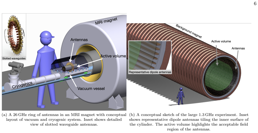
The paper's central claim is that a free-space CRES detector—electrons radiating in a magnetic bottle trap, observed by a cylindrical array of antennas—can collect enough signal to make a $40\ \mathrm{meV}/c^2$ neutrino mass measurement statistically plausible. Each 18.6 keV endpoint electron radiates only about a femtowatt, and antennas cover only part of the solid angle, but the paper shows through simulation that matched-filter detection over many antenna channels recovers sufficient signal-to-noise. The example design uses a 50 mT field, a flat-bottomed trap formed by two coils, and 50,000 dipoles; its projected sensitivity reaches 40 meV at a mean track length of 3 ms (atom density $3.8\times10^{16}\ \mathrm{m}^{-3}$), with longer tracks reaching similar sensitivity at lower background. The authors present the estimate as a benchmark for future CRES efforts, noting that the engineering of such a large array—roughly 50,000 antennas and $O(20\ \mathrm{TB/s})$ data rates—is not yet realized.
Load-bearing premise
The simulation's predictions of signal-to-noise and energy resolution for real trapped electrons are benchmarked only against a static, bench-top 26 GHz source, so the leap to dynamic 18.6 keV electrons in a 0.05 T trap over a 250 m$^3$ volume is untested.
Editorial extensions
If this is right
- CRES would no longer be confined to waveguide-scale active volumes; free-space antenna arrays make cubic-meter-scale detectors in principle possible.
- At the reference operating point, a mean track length of 3 ms—corresponding to a tritium atom density of $3.8\times10^{16}\ \mathrm{m}^{-3}$—is enough to reach the 40 meV sensitivity target.
- At 0.05 T the frequency chirp is slow enough that event-wise energy resolution follows the $\tau^{-3/2}$ scaling of a pure chirp model, so longer trapping times directly improve the mass limit.
- The same analysis pipeline maps antenna choice, trap shape, background rate, and gas density into a sensitivity projection, allowing designs to be compared before building hardware.
- Because the bench measurements bound unmodeled multipath and receiver phase losses at roughly 10%, the simulation-based extrapolation carries a quantified, modest experimental correction.
Reading between the lines
- The largest untested step is the leap from a static bench-top source to real moving electrons: axial motion, Doppler shifts, and the frequency chirp are simulated but not yet measured, so a small 0.05 T trap with a few antennas and a calibrated electron source would be the decisive check.
- If the extrapolation holds, the same free-space antenna-array architecture could be reused for other CRES-style spectroscopies—for example precision beta-decay or x-ray measurements—because the detector volume is decoupled from the operating frequency.
- The $O(20\ \mathrm{TB/s})$ raw data rate suggests that practical realization will hinge on trigger efficiency and online data reduction at least as much as on antenna physics; passive combining of antennas, mentioned but not analyzed in depth here, may be needed to make the channel count tractable.
- The 40 meV projection assumes the endpoint is known and neglects systematic energy smearing; the paper itself shows that additional broadening above roughly 10 meV would spoil the target, so a realistic experiment would need a dedicated calibration strategy.
Signed reviews
Editorial analysis
A structured set of objections, weighed in public.
Referee Report
Summary. The manuscript presents a design study for a free-space cyclotron radiation emission spectroscopy (CRES) detector based on large antenna arrays, aimed at a tritium endpoint neutrino mass measurement. It develops the phenomenology of trapped-electron radiation, describes the CRESana simulation package, validates antenna array performance with bench-top measurements at 26 GHz using a static synthetic source, and combines matched-filter detection with Asimov maximum-likelihood estimation to derive event-wise SNR and energy resolution. These performance parameters feed an analytic sensitivity model that yields a projected limit m_beta < 0.04 eV/c^2 for a 0.05 T, ~250 m^3 active volume with 50,000 dipole antennas and a mean track length of 3 ms. The paper explicitly labels the design idealized and lists several idealizations, including an idealized likelihood reconstruction and the engineering infeasibility of the full array.
Significance. The paper is a useful and comprehensive reference for antenna-array CRES. Its strengths include a complete, openly available simulation chain (CRESana, DOI 10.5281/ZENODO.13935567), bench-scale validation with sub-millimeter position reconstruction and quantified array power losses (15% for the synthetic array, 23% for the full array), and a transparent sensitivity model with explicit idealizations. If the 40 meV projection is taken as a model-derived upper bound, it provides a concrete benchmark for future CRES designs. The main caveat is that the projection relies on a dynamic signal model that is validated only partially, and on an Asimov likelihood that uses the same model for both data and template.
major comments (3)
- [Section VI B and VII A, Eqs. (37)-(38)] The Asimov likelihood analysis uses the CRESana signal model for both the synthetic data x = s(theta_true) + n and the template s(theta) in the likelihood. The event-wise energy resolution quoted in Section VII A is therefore an in-model estimate: any error in the modeled radiation (Eq. 17), the retarded-time phase integral (Eq. 23), or the antenna response cancels between data and model and cannot appear in the quoted resolution. Section VIII C 1 discloses the idealized likelihood reconstruction, but it does not list this data/template self-consistency as an idealization. Since Figure 24 shows that a factor of 1.5 in energy resolution moves the sensitivity from 40 meV to 43 meV at the nominal background, the headline claim is sensitive to exactly this unquantified effect. Please either validate the dynamic signal model against a moving source or an end-to-end measurement, or add a quantitative assessment of the sensitivity to model mismatch, and list this as an idealization in Section VIII C.
- [Section V D and VIII B, Eqs. (35) and (40)] The measured mean power loss of 15% (synthetic array) and 23% (full array) from uncorrected phase errors, antenna-to-antenna differences, and multipath is not propagated into the sensitivity projection of Section VIII B. Because the SNR is proportional to Pdet (Eq. 35) and the event-wise energy resolution scales as SNR^(-1/2) (Eqs. 40-42), a 23% power loss would degrade the ensemble energy resolution and effective volume; the paper should either include this loss as a factor in the simulated Pdet or explicitly estimate its impact on the 40 meV figure.
- [Section V and VIII C] The bench-scale validation in Section V uses a static SYNCA source at 26 GHz, and the paper itself states that 'the SYNCA is a static source and therefore does not address the aforementioned spectral features.' Consequently, the measurements exercise antenna gain, phase, and multipath losses, but they do not test the dynamic 1.3 GHz signal model used for the 0.05 T projection: the retarded-time phase integral of Eq. 23, the Doppler and axial-modulation sidebands, or drift-induced phase shifts. This is the weakest load-bearing link between the prototype and the full-scale sensitivity because Eqs. 35, 36, and 47 all inherit the event-wise SNR and resolution computed from that dynamic model. Section VIII C should list this as an idealization and, ideally, propose a dynamic-source test (for example, a rotating or moving synthetic source, or a small-scale 1.3 GHz validation) that would bound the model error before the 40 meV figure is used as a design benchmark.
minor comments (5)
- [Section VII B 2] The text reads 'the detection efficiency is assumed to be uneffected by start time'; 'uneffected' should be 'unaffected'.
- [Section IV C 2 and Figure 7] The quoted phase error of roughly 2% relative to 2*pi is not translated into an equivalent frequency or energy uncertainty; a one-sentence estimate would help the reader judge the impact on the energy resolution.
- [Section VII B 1, Eq. (44)] The constant constbgd is used in Eq. (44) before it is defined; consider defining it immediately after Eq. (43) or in the sentence preceding Eq. (44).
- [Section II B] The statement that the fraction of kinetic energy in the drift motion is insignificant is plausible, but a quantitative comparison of drift velocity to v_perp and v_parallel would strengthen the justification for neglecting drift in the radiation model.
- [Figures 9-12 and Section IV E] The spectral feature figures are all 'adapted from [10]' without listing the exact simulation parameters in the text; citing the thesis for the precise trap and antenna configurations would improve reproducibility for readers who do not have access to [10].
Circularity Check
No significant circularity: the sensitivity projection is a disclosed, model-based forecast; the in-model Asimov resolution is not presented as an end-to-end measurement, and the bench-scale SYNCA measurements independently anchor the antenna-response component.
full rationale
Walking the derivation chain, the event-wise SNR and energy resolution are computed from the CRESana simulation of the classical electrodynamics signal model (Equations 17, 22, 27, 35, 41), then propagated through Equations 46, 47, and 50 to obtain the projected neutrino mass sensitivity. This is a conditional, simulation-based forecast rather than an empirical measurement: no parameter is fitted to a subset of data and then renamed as a prediction. The only point where data and model coincide is the Asimov likelihood analysis in Section VI B, where the paper states that 'x = s(θtrue) + n, where s(θ) in both the data and the likelihood function is provided by the CRESana simulation tool described in Section IV.' The resulting energy resolution is therefore the Cramer-Rao-style limit of the assumed model, not an end-to-end measurement. The paper is transparent about this: it describes the result as an idealized 'true physical limit' and notes in Section VIII C 1 that a real reconstruction algorithm 'does not know the true minimum and thus will result in larger event-wise energy resolutions.' That is an acknowledged idealization, not a hidden circularity. The prototype measurements in Section V independently benchmark antenna gain, phase, and position reconstruction against a synthetic CRES source; the paper itself admits that 'SYNCA is a static source and therefore does not address the aforementioned spectral features,' so the unvalidated dynamic signal model is a genuine validation gap and correctness risk, but not a circular derivation. The cited prior work, including the CRESana thesis [10] and the chirp CRLB discussion [32], supplies implementation details and context, but the core equations are derived in-text or from standard references such as Jackson and Friis, so no load-bearing self-citation chain forces the conclusion. Accordingly, no circular step meeting the evidence standard is present.
Assumptions & free parameters
free parameters (6)
- System noise temperature T =
5 K
- Background normalization constbgd =
1 s-1 eV-1
- Analysis cuts =
pitch angle > 85 degrees, radius < 1.5 m
- Mean track length <tau> =
3 ms (atom density 3.8e16 m-3)
- Dipole antenna model parameters =
peak gain 3 dB, E-plane pattern [cos((pi/2) sin xi)/cos xi]^2, H-plane constant
- Trap coil configuration =
R_coil=2 m, z=+/-20 m, 2500 amp-turns
assumptions (6)
- domain assumption Adiabatic invariance (v_perp^2/B constant) and rotational symmetry of the magnetic field
- domain assumption Guiding center approximation for electron motion
- domain assumption First-harmonic detection with relativistic corrections
- standard math Friis transmission equation and idealized antenna response
- domain assumption Additive white Gaussian noise model (Nyquist-Johnson)
- domain assumption Known endpoint and Poisson statistics in the sensitivity model
Cite this review
Pith. "Pith review of Antenna Arrays for CRES-based Neutrino Mass Measurement." pith.science (2026). https://pith.science/paper/BDXOQ434
@misc{pith2026250415387,
  author       = {Pith},
  title        = {Pith review of: Antenna Arrays for CRES-based Neutrino Mass Measurement},
  year         = {2026},
  howpublished = {\url{https://pith.science/paper/BDXOQ434}},
  note         = {Machine review of arXiv:2504.15387}
}
abstract
CRES is a technique for precision measurements of kinetic energies of charged particles, pioneered by the Project 8 experiment to measure the neutrino mass using the tritium endpoint method. It was recently employed for the first time to measure the molecular tritium spectrum and place a limit on the neutrino mass using a cm$^3$-scale detector. Future direct neutrino mass experiments are developing the technique to overcome the systematic and statistical limitations of current detectors. This paper describes one such approach, namely the use of antenna arrays for CRES in free space. Phenomenology, detector design, simulation, and performance estimates are discussed, culminating with an example design with a projected sensitivity of $m_{\beta} < 0.04 \ \mathrm{eV}/c^2$. Prototype antenna array measurements are also shown for a demonstrator-scale setup as a benchmark for the simulation. By consolidating these results, this paper serves as a comprehensive reference for the development and performance of antenna arrays for CRES.
Figures


Figures from the paper (21 more)



Reference graph
Works this paper leans on
-
[1]
Retarded Time Since the electron is in motion, Equation 17 is eval- uated at the retarded time tr, defined in Equation 12 wherer is the antenna position and rs is the electron’s position. To solve this equation we simulate the electron trajectory at twice the sampling rate and calculate the delay time to all antennas at each trajectory sample. The delay t...
-
[2]
Power For determining the power incident on an antenna, we use the Friis transmission equation [22]. Assuming unity receiver gain for now (the antenna response is treated in the next section), the power is PEj(t) = PLarmorGe c 2ωc|d| 2 trj(t) , (22) where Ge denotes the electron’s “transmitter gain.” All symbols are evaluated at the retarded time. The gai...
-
[3]
Phase Finally, the instantaneous field phase at each antenna is given as the integral over all past instantaneous field frequencies: φj(t) = Z trj(t) 0 ωc(trj(t′)) dt′ +φc +ϕa(trj(t)). (23) The Doppler shift of the cyclotron frequency is included through a coordinate transformation to the retarded time [10]. In addition to the frequency integral, Equa- ti...
-
[4]
Polarization Mismatch Antennas are only sensitive to radiation polarized in a fixed direction ˆpa, hence the instantaneous electric field E(t) that drives the antenna is the component of Er(t) that is parallel to ˆpa withE(t) = ˆpa·Er(t). For example, the five-slot antenna polarization vector ˆpa is in the same plane as the slots but oriented orthogonal t...
-
[5]
We use HFSS to obtain the trans- fer function for use in the CRES simulation
Frequency response The frequency response is given by the antenna’s trans- fer function defined as H(ω) = U(ω) E(ω), (26) which relates the input electric fieldE to the output volt- ageU at frequency ω. We use HFSS to obtain the trans- fer function for use in the CRES simulation. By design, the bandwidth for the antennas under consideration is wider than ...
-
[6]
Directional response The antenna’s directivityD( ˆd) describes its directional response in the form of a power damping factor. Figure 8 shows howD( ˆd) changes the overall antenna gain of the five-slot antenna in the E and H-plane at a frequency 11 (a) 3D render from HFSS to show the physical orientation of the radiation pattern relative to the antenna. (...
-
[7]
Combined antenna response Combining all the aspects discussed above, the output power of a single antenna element is calculated using the antenna polarization, directivity and the transfer func- tion gain shape: Pout(t) =Mpol(t)·D( ˆd(t))·G(ω0)·PE(t), (27) depending on the input radiation power at the antenna PE, the direction of the source ˆd, and the po...
-
[8]
Synthetic Single-Antenna Array Setup First, a single receiver antenna was placed at a fixed distance from the SYNCA, which was mounted on a ro- tary and translation stage. This single receiver antenna was used to simulate a full array by rotating the SYNCA through a full 360 ◦ rotation at multiple off-axis radial positions (0 to 35 mm from axial center in...
Show all 58 references
-
[9]
A photo of the experimental setup is shown in Figure 13
Full Array Setup To measure physical array effects, bench-top measure- ments were then taken for a full ring of 60 antennas using a Keysight FieldFox vector network analyzer. A photo of the experimental setup is shown in Figure 13. For a given position of the SYNCA source, eac...
-
[10]
Since the SNR is also proportional to the de- tected powerPdet, it depends on the kinetic energy
Signal to Noise Ratio The definition of SNR is given in Equation 35, which shows that the SNR should scale linearly with track length. Since the SNR is also proportional to the de- tected powerPdet, it depends on the kinetic energy. The dependence on kinetic energy comes from ...
-
[11]
whereδω is slope from Equation 29
Event-wise Energy Resolution In a generic chirp model, as discussed in [32], the Cram´ er–Rao lower bound (CRLB) can be calculated for the variance of the initial frequency, which is 1 Var(ˆω0)≥δω2Var(ˆt0) + 192 SNR·τ 2 (40) 1 Note that in the given reference constant in the e...
-
[12]
For the matched filter trigger approach (see Section VI A), the noise distribution from pure white noise is given by a χ2-distribution with two degrees of freedom
Background Rate The background rate is the rate of background events in a specific region of the analysis spectrum, the region of interest ∆EROI. For the matched filter trigger approach (see Section VI A), the noise distribution from pure white noise is given by a χ2-distribut...
-
[13]
The total detec- tion efficiency can be decomposed into the efficiency of trapping an electron and the efficiency of triggering on the received signal
Effective Volume The effective volume Veff is the detection efficiency in- tegrated over the full volume weighted by the probability densities of the electron signal parameters Veff = ZZZ ϵtrap(ρ,z,α∗)·ϵtrig(ρ,α 0,τ|γ) ·P (τ)·P (α0) dα0 dτ dV (45) which is equivalent to the av...
-
[14]
analysis window
Ensemble Energy Resolution The ensemble energy resolution can be calculated by a weighted average, where the weighting factor is pro- portional to the event rate, which is proportional to the effective volume. Thus the ensemble weighted energy res- olution can be defined as ∆E...
-
[15]
In the likelihood reconstruction, the uncertainties are esti- mated from the likelihood profile around the true mini- mum
Idealized likelihood reconstruction The likelihood reconstruction described in Section VI B is used to estimate the event-wise energy resolution. In the likelihood reconstruction, the uncertainties are esti- mated from the likelihood profile around the true mini- mum. However,...
-
[16]
An increase in constbgd can be compensated by requiring a higher anal- ysis threshold
Background rate In Section VII B the dependence of the background rate on the number of independent templates was dis- cussed, and a constant of 1 eV −1 s−1 was used for the neutrino mass sensitivity estimates. An increase in constbgd can be compensated by requiring a higher a...
-
[17]
However, the impact on neutrino mass sensitivity can be tested by adding a non- zero ∆Eother in Equation 49
Additional Contributions to Energy Resolution Additional contributions to the energy resolution have numerous origins and a detailed discussion of them is outside the scope of this paper. However, the impact on neutrino mass sensitivity can be tested by adding a non- zero ∆Eot...
-
[18]
While dipole antennas are some of the simplest antennas, the antenna gain and directivity may influence the performance and the neutrino mass sensitivity
Dipole Antennas The sensitivity was calculated using idealized dipole antennas. While dipole antennas are some of the simplest antennas, the antenna gain and directivity may influence the performance and the neutrino mass sensitivity. To estimate the effect of antenna choice, ...
-
[19]
Precision Physics, Fundamental Interactions, and Structure of Matter
Realization of Setup While this section demonstrates how an antenna ar- ray can be used to reach a neutrino mass sensitivity of 40 meV, surpassing the range allowed by the inverted mass ordering, we have not included the engineering as- pects of the experiment. A physical ante...
-
[20]
Aker et al
M. Aker et al. (Katrin), Direct neutrino-mass mea- surement based on 259 days of KATRIN data (2024), arXiv:2406.13516 [nucl-ex]
2024
-
[21]
Aker et al
M. Aker et al. (KATRIN), J. Phys. G 49, 100501 (2022), arXiv:2203.08059 [nucl-ex]
2022 arXiv
-
[22]
Monreal and J
B. Monreal and J. A. Formaggio, Phys. Rev. D 80, 051301 (2009)
2009
-
[23]
Ashtari Esfahani et al
A. Ashtari Esfahani et al. (Project 8), J. Phys. G 44, 054004 (2017), arXiv:1703.02037 [physics.ins-det]
2017 arXiv
-
[24]
D. M. Asner et al. (Project 8), Phys. Rev. Lett. 114, 162501 (2015)
2015
-
[25]
Ashtari Esfahani et al
A. Ashtari Esfahani et al. (Project 8), Phys. Rev. Lett. 131, 102502 (2023)
2023
-
[26]
Ashtari Esfahani et al
A. Ashtari Esfahani et al. (Project 8), Phys. Rev. C 109, 035503 (2024)
2024
-
[27]
Ashtari Esfahani et al
A. Ashtari Esfahani et al. (Project 8), Phys. Rev. C 99, 055501 (2019)
2019
-
[28]
J. D. Jackson, Classical Electrodynamics, 3rd ed. (John Wiley & Sons, Nashville, TN, 1998)
1998
-
[29]
Thomas, Detection and Estimation Limits of Single Electron Cyclotron Radiation with Phased Array Anten- nas, Ph.D
F. Thomas, Detection and Estimation Limits of Single Electron Cyclotron Radiation with Phased Array Anten- nas, Ph.D. thesis, Johannes Gutenberg University Mainz (2024)
2024
-
[30]
P. O. Vandervoort, Ann. Phys. 10, 401 (1960)
1960
-
[31]
T. G. Northrop, Rev. Geophys. 1, 283 (1963)
1963
-
[32]
Johner, Phys
J. Johner, Phys. Rev. A 36, 1498 (1987)
1987
-
[33]
B. A. Trubnikov, Dokl. Akad. Nauk SSSR 118, 913 (1958)
1958
-
[34]
Ashtari Esfahani et al
A. Ashtari Esfahani et al. (Project 8), J. Instrum. 18 (01), P01034
-
[35]
A. A. Esfahani et al. (Project 8), in Snowmass 2021 (2022) arXiv:2203.07349 [nucl-ex]
2022 arXiv
-
[36]
C. A. Balanis, Antenna Theory: Analysis and Design , 2nd ed. (John Wiley & Sons, 1997)
1997
-
[37]
D. M. Pozar, Microwave engineering , 2nd ed. (Wiley, Hoboken, NJ, 2005)
2005
-
[38]
Elliott and L
R. Elliott and L. Kurtz, IEEE Trans. Antennas Propag. 26, 214 (1978)
1978
- [39]
-
[40]
Simpson, J
J. Simpson, J. Lane, C. Immer, and R. Youngquist, Sim- ple Analytic Expressions for the Magnetic Field of a Cir- cular Current Loop , Tech. Rep. (NASA Technical Re- ports Server (NTRS), 2001)
2001
-
[41]
R. C. Johnson and H. Jasik, Antenna Engineering Hand- book, 2nd ed. (McGraw-Hill, New York, NY, 1984)
1984
-
[42]
H. G. Booker, J. Inst. Electr. Eng - Part IIIA: Radiolo- cation 93, 620 (1946)
1946
-
[43]
Faruque, Radio Frequency Modulation Made Easy (Springer International Publishing, 2017)
S. Faruque, Radio Frequency Modulation Made Easy (Springer International Publishing, 2017)
2017
-
[44]
Ashtari Esfahani et al
A. Ashtari Esfahani et al. (Project 8), J. Instrum. 19 (05), P05073
-
[45]
S. M. Kay, Fundamentals of Statistical Signal Processing, Volume II: Detection theory (Prentice-Hall, 1998)
1998
-
[46]
Van Den Broeck, D
C. Van Den Broeck, D. A. Brown, T. Cokelaer, I. Harry, G. Jones, B. S. Sathyaprakash, H. Tagoshi, and H. Taka- hashi, Phys. Rev. D 80, 024009 (2009)
2009
-
[47]
Babak, R
S. Babak, R. Balasubramanian, D. Churches, T. Coke- laer, and B. S. Sathyaprakash, Classical Quantum Grav- ity 23, 5477 (2006)
2006
-
[48]
Ziegler, Development of Scalable Approaches to Neu- trino Mass Measurement with the Project 8 Experiment , Ph.D
A. Ziegler, Development of Scalable Approaches to Neu- trino Mass Measurement with the Project 8 Experiment , Ph.D. thesis, Pennsylvania State University (2023)
2023
-
[49]
S. S. Wilks, Ann. Math. Stat. 9, 60 (1938)
1938
-
[50]
Cowan, K
G. Cowan, K. Cranmer, E. Gross, and O. Vitells, Eur. Phys. J. C 71, 1 (2011), 1007.1727
2011 arXiv
-
[51]
Buzinsky, Statistical Signal Processing and Detector Optimization in Project 8 , Ph.D
N. Buzinsky, Statistical Signal Processing and Detector Optimization in Project 8 , Ph.D. thesis, Massachusetts Institute of Technology (2021)
2021
-
[52]
J. A. Formaggio, A. L. C. de Gouvˆ ea, and R. G. H. Robertson, Phys. Rep. 914, 1 (2021)
2021
-
[53]
Ashtari Esfahani et al
A. Ashtari Esfahani et al. (Project 8), Phys. Rev. C 103, 065501 (2021)
2021
-
[54]
Iwasaki, A
Y. Iwasaki, A. Tan, and C. G. Tully (PTOLEMY), To- wards CRES-Based Non-destructive Electron Momen- tum Estimation for the PTOLEMY Relic Neutrino De- tector (2024), arXiv:2404.00817 [physics.ins-det]
2024 arXiv
-
[55]
Farino et al
M. Farino et al. (PTOLEMY), A Demonstration of Slowed Electron E × B Drift for PTOLEMY (2025), arXiv:2503.10025 [physics.ins-det]
2025 arXiv
-
[56]
A. A. S. Amad et al., Determining absolute neutrino mass using quantum technologies (2024), arXiv:2412.06338 [hep-ex]
2024
-
[57]
Byron et al
W. Byron et al. (He6-CRES), Phys. Rev. Lett. 131, 082502 (2023)
2023
-
[58]
Kazkaz and N
K. Kazkaz and N. Woollett, New J. Phys. 23, 033043 (2021)
2021
Reviewed August 16, 2026 · model on record in the stance chip above.
Discussion (0). Continue with ORCID to comment.