Learning functions of Hamiltonians with Hamiltonian Fourier features

Akimoto Nakayama; Hidetaka Manabe; Kosuke Mitarai; Yuto Morohoshi

REVIEW 3 major objections 4 minor 24 references

Learning functions of Hamiltonians with Hamiltonian Fourier features

T0 review · 3 major / 4 minor · reviewed 2026-08-16 · deepseek-v4-flash

Challenge this review Re-run · record.json Download PDF Read on arXiv ↗ Review JSON

Pith's one-line read The paper proves that learning an unknown function of a Hamiltonian inside the expression $\mathrm{Tr}[f(H)\rho]$ is provably easy for quantum computers, with explicit polynomial feature and sample counts, and demonstrates the linear…

desk verdict A genuinely new QML task with a clean Rademacher bound, but the headline corollary overclaims: the Fourier feature map is periodic, so Lipschitz functions without matching endpoint values break the guarantee. read the letter →

arxiv 2504.16370 v2 pith:4B2363BG submitted 2025-04-23 quant-ph

Yuto Morohoshi , Akimoto Nakayama , Hidetaka Manabe , Kosuke Mitarai This is my paper · ORCID

classification quant-ph PACS 03.67.Lx

keywords quantummachinelearningHamiltonianFourierfeatureslinearregressionseriesapproximationsamplecomplexitysimulationsuperconductingqubitsgeneralizationbound

verification ladder T0 review T1 audit T2 compute T3 formal

The pith

A machine-rendered reading of the paper's core claim, the machinery that carries it, and where it could break.

The reading

This paper proposes a machine-learning task, predicting $y=\mathrm{Tr}[f(H)\rho]$ from descriptions of $H$ and $\rho$ when $f$ is unknown, and claims that the task is provably easy for a quantum computer whenever $f$ has a rapidly converging Fourier series on $[-C,C]$. The learner uses Hamiltonian Fourier features, the real and imaginary parts of $\mathrm{Tr}[e^{-il\pi H/C}\rho]$, and fits a linear model by regression. The main theorem bounds expected squared loss by a Fourier truncation term plus a sample-size term; for Lipschitz $f$ this gives $K=O(\log(1/\varepsilon)/\varepsilon)$ features and $N_d=O((W\|f\|_\infty \log(1/\varepsilon)/\varepsilon)^4)$ samples to reach error $\varepsilon$. The same guarantee is shown to survive bounded measurement noise with polynomially many shots, and the paper reports experimental regressions on a superconducting processor at 12, 32, and 40 qubits, with the two smaller systems reaching high test $R^2$ and the 40-qubit run dominated by device noise. The practical interest is that this is one of the few concrete learning problems with a polynomial quantum sample-complexity proof and a plausible, though not rigorous, classical-hardness argument.

What carries the argument

The load-bearing object is the Hamiltonian Fourier feature vector $x(H,\rho)=(x_0,\ldots,x_{2K})$, whose even entries are $\mathrm{Re}\,\mathrm{Tr}[e^{-il\pi H/C}\rho]$ and odd entries are $\mathrm{Im}\,\mathrm{Tr}[e^{-il\pi H/C}\rho]$ for $l=0,\ldots,K$. These features are the Fourier coefficients of the spectral measure of $H$ against $\rho$, so the linear model $g=w\cdot x$ is a truncated Fourier series in the eigenvalues of $H$. The key properties that make the proof work are that each feature has magnitude at most 1, so the feature Gram matrix has trace at most $(2K+1)N_d$, and that the constrained weight class $\{w^Tw\le W^2\}$ has a tractable generalization bound; this separates the approximation error, controlled by the Fourier truncation $\varepsilon_K$, from the estimation error, controlled by the sample count $N_d$. The same machinery extends to noisy features by adding a deterministic term linear in the per-feature noise level $\eta$.

What would settle it

A direct test is to seek a classical polynomial-time algorithm that estimates $\mathrm{Tr}[\cos(tH)\rho]$ for random few-body Hamiltonians with $t=\mathrm{poly}(n)$; if such an algorithm exists, the argued quantum advantage collapses. A second test is to find a Lipschitz $f$ satisfying the theorem's hypotheses whose actual required $K$ and $N_d$ outgrow the stated polynomial bounds, which would contradict Corollary 1.

Watch

Extended reading notes

Core claim

The central discovery is that $f(H)$ inside a trace can be learned by expanding it as a Fourier series in the eigenvalues of $H$ and using quantum-evolution expectation values as features. Concretely, Theorem 1 states that for any $f$ admitting a uniform Fourier approximation on $[-C,C]$ with coefficient norm bound $W$, the minimizer of empirical squared loss over the linear model $g(H,\rho;w)=w\cdot x(H,\rho)$ with $x(H,\rho)$ built from real and imaginary parts of $\mathrm{Tr}[e^{-ik\pi H/C}\rho]$ achieves expected loss bounded by $\varepsilon_K^2$ plus generalization terms that go to zero as the sample count $N_d$ grows. Corollary 1 specializes this to Lipschitz $f$, where $\varepsilon_K=O(\log K/K)$, so $K=O(\log(1/\varepsilon)/\varepsilon)$ and $N_d=O((W\|f\|_\infty\log(1/\varepsilon)/\varepsilon)^4)$ suffice for expected loss at most $\varepsilon$. The proof bounds every feature by 1, uses a standard generalization bound for constrained linear models, and notes that the empirical loss at the Fourier coefficients is at most $\varepsilon_K^2$. Theorem 2 extends the result to noisy features, requiring $O(\log(K/\delta)/\eta^2)$ shots per feature, and the hardware experiments with $f(H)=e^{-\beta H}$ use a reference-eigenstate identity to measure features without controlled time evolution.

Load-bearing premise

The quantum-easiness guarantee holds only for functions $f$ whose expansion into sine and cosine waves on $[-C,C]$ converges quickly and has bounded total squared weight; for functions with slowly decaying expansion coefficients, neither the stated feature count nor the stated sample count is guaranteed to be enough.

Editorial extensions

If this is right

For Lipschitz-continuous $f$, any target error $\varepsilon$ is reached with $K=O(\log(1/\varepsilon)/\varepsilon)$ features and $N_d=O((W\|f\|_\infty\log(1/\varepsilon)/\varepsilon)^4)$ samples, placing the task among the few supervised learning problems with a polynomial quantum sample-complexity guarantee.
Because the features are values of time evolution generated by $H$, choosing $f(H)=\cos(tH)$ or $\sin(tH)$ makes the learned label a Hamiltonian-simulation output; if simulation of such Hamiltonians is classically hard, the task provides a learning separation with practical-looking instances.
The reference-eigenstate identity used in the experiments lets features be obtained without controlled time evolution for Hamiltonians with a known eigenstate orthogonal to the input state, which is what allows near-term demonstrations on current devices.
The noise analysis says that estimating each feature with $O(\log(K/\delta)/\eta^2)$ shots is enough to keep the expected-loss guarantee polynomial, so the protocol remains learnable under finite measurement statistics.
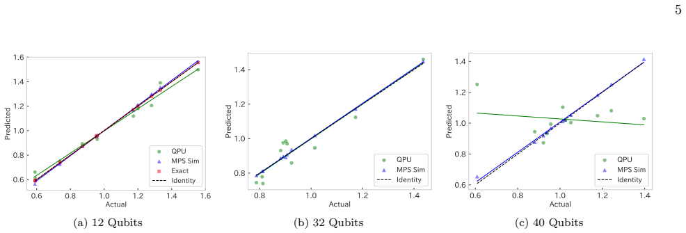
In the reported demonstrations, the 12- and 32-qubit regressions achieve test $R^2$ above 0.8, while the 40-qubit run gives no meaningful prediction, indicating device noise rather than the learning model as the practical bottleneck.

Reading between the lines

Editorial extensions of the paper, not claims the author makes directly.

Editorial inference: the feature vector defines a kernel $K((H,\rho),(H',\rho'))=x(H,\rho)^T x(H',\rho')$, so the same construction could be reused for kernel-based learning of other Hamiltonian-dependent targets; the paper does not pursue this.
Editorial inference: the $W^4$ dependence in the sample bound is the quantity most likely to become impractical as $f$ becomes less smooth; testing the method on a sharp-cornered Lipschitz function with a large Fourier coefficient norm would map where the provable-easiness guarantee stops being useful in practice.
Editorial inference: the classical-hardness argument is informal because it relies on worst-case simulation hardness, so a rigorous separation would need average-case hardness over the training distribution; a concrete route is to instantiate the task with Hamiltonians that encode a quantum computation believed hard on average, a direction the paper mentions but leaves open.

Share X Bluesky LinkedIn Reddit HN

Signed reviews

No signed human review yet.

Editorial analysis

A structured set of objections, weighed in public.

Desk editor's note, referee report, and a circularity audit.

Desk Editor's Note

read the letter

Good to see this one. The core idea is genuinely new: learning an unknown function f in y = Tr[f(H)rho] from Hamiltonian descriptions, using time-evolved features and a linear model with a Rademacher generalization bound. That's a clean QML task with a polynomial sample guarantee, and the authors are honest that classical hardness remains open. The noise-robustness appendix is a plus, and the code is released.

But there is a load-bearing error in the statement of Corollary 1. The feature map is 2C-periodic in the eigenvalues of H, so any linear model over these features is 2C-periodic when viewed as a function of those eigenvalues. For a Lipschitz f with f(-C) != f(C), the truncated Fourier series cannot approximate f uniformly on [-C,C]; the classic O(log K/K) convergence applies to periodic functions, not to arbitrary Lipschitz functions on a closed interval. The counterexample is concrete: take C=1, f(x)=x, rho=|0><0|, and p uniform over H=+I and H=-I. Then x_cos,k = cos(k pi) = (-1)^k and x_sin,k = 0 for both H, so the two samples have identical features but labels +1 and -1. No linear model can get expected squared loss below 1, contradicting Corollary 1 for epsilon < 1. This is not cosmetic; it undermines the headline claim of provable easiness for arbitrary Lipschitz f. The fix is standard: assume f is 2C-periodic, or assume the spectral support of H under p is strictly inside (-C,C). The experimental target f(H)=e^{-beta H} on [-3,3] violates the periodicity condition, though it might still satisfy the second condition if the eigenvalue spectra avoid the endpoints.

Other soft spots are minor. The definition of W in Theorem 1 looks dimensionally off: it defines W as an integral of |f|^2 rather than a square root, so the constraint sum c_k^2 <= W^2 is mismatched. Easy to repair, but needs a correction. The 32- and 40-qubit experiments use ExtraTrees, not the linear model from the proof, so the QPU results do not actually demonstrate the proved model. The 40-qubit failure is reported transparently, which I credit. The citation pattern is fine; prior separation tasks use different oracles and different targets, so the novelty claim holds.

Overall: a serious paper with a fixable but real flaw in the central claim. I'd send it to peer review with a request for major revision. Once the periodicity condition is added and the experiments are aligned with the model class, this becomes a citeable contribution.

Referee Report

3 major / 4 minor

Summary. The paper proposes a supervised quantum machine learning task: predict y = Tr[f(H)ρ] for an unknown scalar function f, given classical descriptions of an n-qubit Hamiltonian H and state ρ. The proposed learner constructs Hamiltonian Fourier features x_k(H,ρ) = Tr[e^{-ikπH/C}ρ] and fits a linear model g(H,ρ;w) = w·x. The main theoretical result, Theorem 1, is a Rademacher-complexity generalization bound; Corollary 1 claims that for Lipschitz f, K = O(log(1/ε)/ε) features and N_d = O((W∥f∥∞ log(1/ε)/ε)^4) samples suffice to reach expected squared loss ε. Appendix B extends the result to noisy feature estimates. The paper reports experiments on IBM Quantum processors with 12, 32, and 40 qubits for f(H) = e^{-βH}, using a protocol that avoids controlled time evolution.

Significance. If the learnability claim is stated correctly, the task is an interesting candidate for a practically relevant learning problem that is provably easy for quantum computers under a Fourier-expandability assumption. The paper's strengths include a self-contained proof via standard Rademacher-complexity tools, an explicit analysis of finite-shot noise, a hardware demonstration with a useful feature-estimation trick, and publicly available code. However, the current statement of Corollary 1 overreaches because it omits the periodicity condition needed for uniform trigonometric approximation, and the experimental section partially validates a different model class at large sizes. With targeted revisions the central idea is sound and the paper could make a solid contribution.

major comments (3)

[Section II, paragraph after Theorem 1 and Corollary 1] The claim that Lipschitz continuity implies ε_K = O(log K / K) uniformly on [-C,C] is false for functions with f(-C) ≠ f(C), because every 2C-periodic trigonometric polynomial p satisfies p(-C) = p(C). Concretely, take C = 1, f(x) = x, ρ = |0⟩⟨0|, and p uniform over H = +I and H = -I. Equations (3)-(5) give x_{cos,l} = cos(lπ) = (-1)^l and x_{sin,l} = 0 for both H, so the features coincide. Every linear model g(H,ρ;w) = w·x outputs the same value v for both Hamiltonians, while the labels are y = Tr[Hρ] = ±1. The expected squared loss is v² + 1 ≥ 1 for every w, every K, and every N_d, so Corollary 1's conclusion R(w*) ≤ ε fails for any ε < 1. The experimental target f(H) = e^{-βH} with C = 3 also has e^{-3} ≠ e^3 and therefore falls outside the stated assumption. A corrected statement should either require f to be 2C-periodic, or assume that the distribution's spectral support is strictly inside (-C,C) with a margin δ > 0 and make the bound depend explicitly on δ.
[Theorem 1, Section II; Appendix A, Lemma 3] The definition of W is dimensionally inconsistent with its use. The theorem defines W = (1/(2C))∫_{-C}^{C} |f(x)|² dx, which has units of f², but then imposes the weight constraint w^T w ≤ W² and uses W linearly in the bound (7). Under a global scaling f → α f, the right-hand side of (7) would scale as α³ instead of the correct α². The consistent definition is W = sqrt((1/(2C))∫_{-C}^{C} |f(x)|² dx), or another suitable norm of f, and this correction propagates to the sample-complexity expression in Corollary 1 and to Lemma 3. This appears to be a typographical slip, but it must be fixed for the quantitative claims to be meaningful.
[Section III, Table I and Fig. 2] The experimental validation of the proposed linear model (6) is limited to 12 qubits. At 32 and 40 qubits, the QPU regression method selected by PyCaret is ExtraTreesRegressor, which is not of the form g(H,ρ;w) = w·x and for which no learning-theoretic guarantee is given in the paper. The 32-qubit QPU result (R² = 0.889) therefore demonstrates that a non-linear classical regressor can fit the data, not that the Hamiltonian Fourier feature model works at that scale. Moreover, the 40-qubit QPU result has R² = -0.430, which the text itself describes as not providing a meaningful prediction. The abstract and introduction state the method is demonstrated 'up to 40 qubits'; this should be qualified to indicate that the linear feature model is validated on hardware only at 12 qubits, while the larger runs are validated in noiseless MPS simulation and fail under current device noise at 40 qubits.

minor comments (4)

[Eq. (3)] The subscript notation in Eq. (3), e.g., 'xcos,k/2', is ambiguous; it should be typeset as x_{cos,k/2} for even k and x_{sin,(k+1)/2} for odd k.
[Theorem 1 statement] The coefficient sequence {c_k}_{k=0}^{2K} is used as c_{2k} and c_{2k+1}, but the indexing is unclear. It would be cleaner to define two separate sequences {a_k}_{k=0}^{K} and {b_k}_{k=0}^{K-1} for the cosine and sine coefficients.
[Section III.B] The statement that the TEBD bond dimension χ=100 'gives values essentially equivalent to the exact value with an error less than 10^{-6} at 12 qubits' verifies only the 12-qubit case; for 32 and 40 qubits, no comparison against exact values is provided, so the accuracy of the labels y_j is not established to the same standard.
[Section II, classical hardness paragraph] The phrase 'strongly believed to be a hard task' understates the status of Hamiltonian simulation: estimating Tr[e^{-itH}ρ] is BQP-complete in the worst case. The genuinely open issue, which the paper correctly identifies, is the average-case hardness needed for the learning separation.

Circularity Check

0 steps flagged · score 0.0 of 10

No significant circularity; the learnability proof is self-contained and reduces to external, standard learning-theory results.

full rationale

Score 0. The core bound in Theorem 1 is not circular: the approximation error ε_K is an explicit assumption on f, and the generalization terms come from standard Rademacher-complexity bounds (Mohri et al., Lemmas 1 and 2) applied to a norm-constrained linear model. The Hamiltonian Fourier features x(H,ρ) are defined independently of f, and the learned weights are fitted to labeled data; the Fourier coefficients of the unknown f are properties of f, not quantities fitted to the experimental target. The experimental labels are generated classically via TEBD and validated against exact simulation, so there is no fitted-input-called-prediction step. The feature-estimation strategy follows the external result [15] through the direct identity in Eq. (8), and the claimed quantum easiness relies on the standard ability to estimate Tr[e^{-iHt}ρ] via Hadamard tests. No load-bearing conclusion is justified solely by the authors' own prior work. A separate mathematical-correctness concern, distinct from circularity, is that Corollary 1's K = O(log(1/ε)/ε) step cites a Fourier-approximation theorem that applies to periodic functions; for general Lipschitz f on [-C,C] with f(C) ≠ f(-C), uniform approximation by trigonometric polynomials cannot converge to zero, as the features for H = ±C collapse. This is a validity issue in the stated corollary, not a circular-derivation issue.

Assumptions & free parameters 4 free parameters · 5 assumptions · 0 invented entities

The central theoretical result rests on standard learning-theory tools and the assumption that the unknown f has a fast-converging Fourier series. The experimental demonstration additionally relies on a reference-eigenstate construction that limits the class of implementable instances. No new physical entities or potential-free parameters are introduced beyond the model hyperparameters and Trotter step choices.

free parameters (4)

K (Fourier truncation order) = 11 (experiment)
Chosen for the experiment; validated by exact simulation achieving R2=1.00. In theory K is set by the desired accuracy epsilon, growing as O(log(1/epsilon)/epsilon) for Lipschitz f.
nstep (Trotter steps) per feature = [1,1,1,1,1,2,2,2,2,3,3,3] (12q), [1,1,2,2,2,2,3,3,3,3,4,4] (32q), [1,1,2,2,2,3,3,4,4,4,5,5] (40q)
Heuristically chosen per feature l to balance Trotter error and circuit depth; no rigorous error analysis is provided in the paper.
Regression model (PyCaret AutoML) = BayesianRidge (12q), ExtraTreesRegressor (32q, 40q)
Selected by PyCaret based on k-fold cross-validation MSE on the training set; the 32- and 40-qubit models are not the linear model class analyzed in Theorem 1.
beta in f(H)=e^{-beta H} = 1
Demonstration choice; not fitted to data, but it sets the smoothness and scale of the labels. The method is not tied to this value.

assumptions (5)

standard math Uniform convergence of Fourier series for Lipschitz functions with error O(log K/K) (used in Corollary 1)
Invoked to set K = O(log(1/epsilon)/epsilon) for a target accuracy epsilon; sourced from Salem and Zygmund [12].
standard math Rademacher complexity and generalization bounds from Mohri et al. [24] (Lemma 1, Lemma 2)
Used in Appendix A to bound the expected loss in terms of empirical loss and Rademacher complexity.
domain assumption Efficient Hamiltonian simulation and state preparation for H and rho in the support of p(H,rho) (Section II)
The quantum algorithm is efficient only if the input Hamiltonians and states have efficient quantum circuit descriptions.
domain assumption The reference-eigenstate overlap formula (Eq. 8) from Kyriienko [15], requiring an efficient classically findable eigenstate |psi_ref> orthogonal to |psi>
Used in the experimental feature-estimation shortcut; restricts the experiment to states and Hamiltonians with such symmetries.
domain assumption The target f admits a bounded-coefficient Fourier expansion (Theorem 1)
The polynomial sample complexity guarantee holds only for functions with uniformly convergent Fourier series on [-C,C] and coefficient norm bounded by W.

how reviews work

0 comments

Cite this review

Pith. "Pith review of Learning functions of Hamiltonians with Hamiltonian Fourier features." pith.science (2026). https://pith.science/paper/4B2363BG

@misc{pith2026250416370,
  author       = {Pith},
  title        = {Pith review of: Learning functions of Hamiltonians with Hamiltonian Fourier features},
  year         = {2026},
  howpublished = {\url{https://pith.science/paper/4B2363BG}},
  note         = {Machine review of arXiv:2504.16370}
}

abstract

We propose a quantum machine learning task that is provably easy for quantum computers and arguably hard for classical ones. The task involves predicting quantities of the form $\mathrm{Tr}[f(H)\rho]$, where $f$ is an unknown function, given descriptions of $H$ and $\rho$. Using a Fourier-based feature map of Hamiltonians and linear regression, we theoretically establish the learnability of the task and implement it on a superconducting device using up to 40 qubits. This work provides a machine learning task with practical relevance, provable quantum easiness, and near-term feasibility.

Figures

Figures reproduced from arXiv: 2504.16370 by the authors.

**Figure 2.** FIG. 2. Demonstration results for 12, 32, and 40 qubits. The horizontal axes represent actual [PITH_FULL_IMAGE:figures/full_fig_p005_2.png] view at source ↗

**Figure 3.** FIG. 3. Comparison between the QPU and the noiseless MPS simulator, which effectively provides exact simulation results. [PITH_FULL_IMAGE:figures/full_fig_p005_3.png] view at source ↗

Figures from the paper (3 more)

**Figure 4.** Figure 4: FIG. 4. Quantum circuit of Hadamard test to estimate [PITH_FULL_IMAGE:figures/full_fig_p010_4.png]

**Figure 5.** Figure 5: FIG. 5. Mapping from logical qubits (green numbers) to physical qubits (white numbers) on [PITH_FULL_IMAGE:figures/full_fig_p011_5.png]

**Figure 6.** Figure 6: FIG. 6. Examples of a logical circuit (before transpilation) and the corresponding physical circuit (after transpilation) used [PITH_FULL_IMAGE:figures/full_fig_p012_6.png]

Discussion (0). Continue with ORCID to comment.

Reference graph

Works this paper leans on

24 extracted references · 11 canonical work pages

[1]

Cerezo, G

M. Cerezo, G. Verdon, H.-Y. Huang, L. Cincio, and P. J. Coles, Nature computational science 2, 567 (2022)

work page 2022
[2]

Biamonte, P

J. Biamonte, P. Wittek, N. Pancotti, P. Rebentrost, N. Wiebe, and S. Lloyd, Nature 549, 195 (2017)

2017
[3]

Cerezo, A

M. Cerezo, A. Arrasmith, R. Babbush, S. C. Benjamin, S. Endo, K. Fujii, J. R. McClean, K. Mitarai, X. Yuan, L. Cincio, and P. J. Coles, Nature Reviews Physics3, 625 (2021)

2021
[4]

R. A. Servedio and S. J. Gortler, SIAM Journal on Com- puting 33, 1067 (2004)

work page 2004
[5]

Kearns and L

M. Kearns and L. Valiant, J. ACM 41, 67–95 (1994)

work page 1994
[6]

Y. Liu, S. Arunachalam, and K. Temme, Nature physics 17, 1013 (2021). 6

work page 2021
[7]

Schuld and N

M. Schuld and N. Killoran, Physical Review Letters 122, 040504 (2019)

2019
[8]

Havl´ ıˇ cek, A

V. Havl´ ıˇ cek, A. D. C´ orcoles, K. Temme, A. W. Harrow, A. Kandala, J. M. Chow, and J. M. Gambetta, Nature 567, 209 (2019)

2019

Show all 24 references

[9]

Yamasaki, N

H. Yamasaki, N. Isogai, and M. Murao, arXiv:2312.03057 [quant-ph] (2023)

2023 arXiv
[10]

Gyurik and V

C. Gyurik and V. Dunjko, arXiv:2306.16028 [quant-ph] (2023)

2023 arXiv
[11]

Molteni, C

R. Molteni, C. Gyurik, and V. Dunjko, arXiv:2405.02027 [quant-ph] (2024)

2024 arXiv
[12]

Salem and A

R. Salem and A. Zygmund, Trans. Amer. Math. Soc. 59, 14 (1946)

1946
[13]

R. P. Feynman, Found. Phys. 16, 507 (1986)

1986
[14]

Cifuentes, S

S. Cifuentes, S. Wang, T. L. Silva, M. Berta, and L. Aolita, arXiv preprint arXiv:2410.13937 (2024)

2024 arXiv
[15]

Kyriienko, npj Quantum Information 6, 7 (2020)

O. Kyriienko, npj Quantum Information 6, 7 (2020)

2020
[16]

Vidal, Physical review letters 93, 040502 (2004)

G. Vidal, Physical review letters 93, 040502 (2004)

2004
[17]

Hauschild, J

J. Hauschild, J. Unfried, S. Anand, B. Andrews, M. Bintz, U. Borla, S. Divic, M. Drescher, J. Geiger, M. Hefel, K. H´ emery, W. Kadow, J. Kemp, N. Kirchner, V. S. Liu, G. M¨ oller, D. Parker, M. Rader, A. Romen, S. Scalet, L. Schoonderwoerd, M. Schulz, T. Soejima, P. Thoma, Y....

2024
[18]

IBM Quantum, https://quantum.ibm.com/ (2025)

2025
[19]

Javadi-Abhari, M

A. Javadi-Abhari, M. Treinish, K. Krsulich, C. J. Wood, J. Lishman, J. Gacon, S. Martiel, P. D. Nation, L. S. Bishop, A. W. Cross, B. R. Johnson, and J. M. Gambetta, Quantum computing with Qiskit (2024), arXiv:2405.08810 [quant-ph]

2024 arXiv
[20]

Vidal, Physical review letters 91, 147902 (2003)

G. Vidal, Physical review letters 91, 147902 (2003)

2003
[21]

Ali, PyCaret: An open source, low-code machine learning library in Python (2020), pyCaret version 1.0

M. Ali, PyCaret: An open source, low-code machine learning library in Python (2020), pyCaret version 1.0

2020
[22]

Z. Cai, R. Babbush, S. C. Benjamin, S. Endo, W. J. Hug- gins, Y. Li, J. R. McClean, and T. E. O’Brien, Reviews of Modern Physics 95, 045005 (2023)

2023
[23]

S. Endo, Z. Cai, S. C. Benjamin, and X. Yuan, Journal of the Physical Society of Japan 90, 032001 (2021)

2021
[24]

KX k=0 w2k cos(kπλi,l/C) + K−1X k=0 w2k+1 sin(kπλi,l/C) # pl !2 (A7) = 1 Nd NdX i=1

M. Mohri, A. Rostamizadeh, and A. Talwalkar, Foun- dations of Machine Learning , 2nd ed. (The MIT Press, Cambridge, MA, 2018) a new edition of a graduate-level machine learning textbook that focuses on the analysis and theory of algorithms. Appendix A: Proof of quantum easines...

2018

Pith tools

Reviewed August 16, 2026 · model on record in the stance chip above.

[1] [1]

Cerezo, G

M. Cerezo, G. Verdon, H.-Y. Huang, L. Cincio, and P. J. Coles, Nature computational science 2, 567 (2022)

work page 2022

[2] [2]

Biamonte, P

J. Biamonte, P. Wittek, N. Pancotti, P. Rebentrost, N. Wiebe, and S. Lloyd, Nature 549, 195 (2017)

2017

[3] [3]

Cerezo, A

M. Cerezo, A. Arrasmith, R. Babbush, S. C. Benjamin, S. Endo, K. Fujii, J. R. McClean, K. Mitarai, X. Yuan, L. Cincio, and P. J. Coles, Nature Reviews Physics3, 625 (2021)

2021

[4] [4]

R. A. Servedio and S. J. Gortler, SIAM Journal on Com- puting 33, 1067 (2004)

work page 2004

[5] [5]

Kearns and L

M. Kearns and L. Valiant, J. ACM 41, 67–95 (1994)

work page 1994

[6] [6]

Y. Liu, S. Arunachalam, and K. Temme, Nature physics 17, 1013 (2021). 6

work page 2021

[7] [7]

Schuld and N

M. Schuld and N. Killoran, Physical Review Letters 122, 040504 (2019)

2019

[8] [8]

Havl´ ıˇ cek, A

V. Havl´ ıˇ cek, A. D. C´ orcoles, K. Temme, A. W. Harrow, A. Kandala, J. M. Chow, and J. M. Gambetta, Nature 567, 209 (2019)

2019