REVIEW 4 major objections 6 minor 38 references
FR-Mamba: Time-Series Physical Field Reconstruction Based on State Space Model
T0 review · 4 major / 6 minor · reviewed 2026-08-07 · deepseek-v4-flash
Pith's one-line read A hybrid of the Mamba state-space model and Fourier neural operators reconstructs unsteady vorticity fields from 16 sparse sensors with roughly one-third the error of the previous best method on the cylinder-flow benchmark.
desk verdict Plausible Mamba+FNO architecture, but the L notation and train split contradictions make the reported benchmark results unreproducible as written. read the letter →
The pith
A machine-rendered reading of the paper's core claim, the machinery that carries it, and where it could break.
The reading
What carries the argument
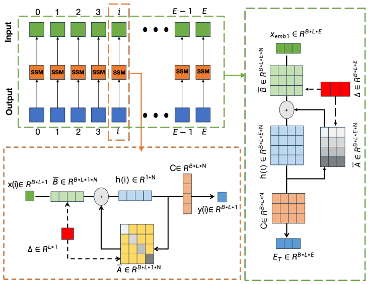
The load-bearing object is the FNO-Mamba block, a dual-branch module with a temporal branch and a spatial branch. The temporal branch is a selective state-space model (Mamba): embeddings produce per-step control matrices $B$ and $C$ and a learnable time step $\Delta$; the continuous transition matrix $A$ is discretized by zero-order hold; and the hidden state is updated recurrently but computed in parallel across feature dimensions, so long-range dependencies are encoded with linear time complexity. The spatial branch is a one-dimensional Fourier neural operator: each sensor channel is transformed with a discrete Fourier transform, only the first $m$ frequency modes are retained, each mode is multiplied by a learnable complex weight matrix $W_k$, and an inverse transform returns a global spatial representation. A gating mechanism fuses the two branch outputs, residual connections stack the blocks, and a 2D Fourier operator with a residual connection refines the final reconstructed field. The ablations show what this machinery is doing: without either Fourier operator, Max-AE is $0.355\times10^{-2}$; the 1D operator alone cuts it to $0.125\times10^{-2}$, and the full model reaches $0.108\times10^{-2}$.
What would settle it
Re-running the identical benchmark with 16 sensors on the $Re=100$ cylinder flow, a single fixed training split (for instance 400 training snapshots), and one consistent sequence length should reproduce FR-Mamba's average MAE near $0.31\times10^{-4}$ and Max-AE near $0.10\times10^{-2}$, with both below PFR-Transformer's $0.91\times10^{-4}$ and $0.53\times10^{-2}$ on every test interval; a reversal of that ordering, or a large shift in the absolute errors, would settle the claim against the paper.
Extended reading notes
Core claim
The central claim is that FR-Mamba is the first state-space-model-based physical field reconstruction method and that it outperforms all compared baselines—SVR-POD, LSTM-POD, Voronoi UNet, Shallow Decoder, Voronoi CNN, Gappy MLP, and PFR-Transformer—on both mean and maximum absolute error for time-series cylinder-flow reconstruction. The authors' key assertion is that temporal context, not just spatial encoding, is what earlier methods miss, and that a selective state-space model supplies that context at linear cost. The reported average errors are $0.31\times10^{-4}$ MAE and $0.10\times10^{-2}$ Max-AE across the five test intervals, compared with $0.91\times10^{-4}$ and $0.53\times10^{-2}$ for PFR-Transformer, with the error staying nearly flat from the first interval to the last. The ablation evidence is part of the claim: removing both Fourier operators raises MAE to $0.397\times10^{-4}$ and Max-AE to $0.355\times10^{-2}$; adding the 1D operator alone brings them to $0.315\times10^{-4}$ and $0.125\times10^{-2}$; adding the 2D operator reaches the final $0.310\times10^{-4}$ and $0.108\times10^{-2}$.
Load-bearing premise
The whole comparison rests on the experiment being run exactly as described—a fixed 16-sensor layout on the $Re=100$ cylinder-flow dataset, one unambiguous training/test split, and the same meaning of sequence length in the temporal branch and the reconstruction head; if any of those conventions differ, the reported error numbers cannot be reproduced or compared.
Editorial extensions
If this is right
- A pure Mamba without spatial encoding is much weaker: removing both Fourier operators raises MAE from $0.310\times10^{-4}$ to $0.397\times10^{-4}$ and Max-AE from $0.108\times10^{-2}$ to $0.355\times10^{-2}$, so frequency-domain spatial modeling is a necessary complement to the state-space model.
- The model's error stays nearly flat across the five test intervals (MAE 0.30–0.32, Max-AE 0.10–0.11), so it does not appear to accumulate error on long sequences the way recurrent baselines do.
- Because the SSM branch runs in linear time, scaling to longer sensor histories should be cheaper than attention-based physical field reconstruction approaches; the paper frames this as the main practical advantage.
- The best configuration found is moderate depth with a compact hidden dimension ($N_{layer}=10$, $D=8$); deeper and wider models degrade, which the paper attributes to overfitting under limited training data.
- The reconstructed quantities are vorticity fields on a fixed 2D grid from a fixed 16-sensor layout, so the method is directly applicable to other physical-field reconstruction problems with the same geometric setup and time-series sensor inputs.
Reading between the lines
- Beyond the paper: the same dual-branch design should transfer to other sparse-sensor PDE fields (pressure, temperature, concentration) whenever the sensor layout is fixed and the output lives on a regular grid, because neither branch assumes cylinder-specific physics.
- Beyond the paper: the flat T1–T5 error suggests the model does not compound error over long sequences within the tested window, but the paper does not test beyond the 1000-snapshot test set; running the trained model on much longer rollouts would show where accumulation eventually begins.
- Beyond the paper: the sharp degradation at $N_{layer}=20$ hints that limited training data, not architecture capacity, is the active constraint on this benchmark, so the reported gap over baselines might grow or shrink with more training snapshots.
- Beyond the paper: pairing the deterministic MAE-trained decoder with a probabilistic head would let the model output uncertainty alongside the field, which is what sensor-based reconstruction needs for engineering decisions.
Editorial analysis
A structured set of objections, weighed in public.
Referee Report
Summary. FR-Mamba is a dual-branch neural architecture for time-series physical field reconstruction from sparse sensor measurements. The temporal branch uses Mamba/SSM to capture long-range dependencies, the spatial branch uses a 1D Fourier Neural Operator, a gating mechanism fuses the two, and a 2D FNO refines the output. The authors evaluate on two-dimensional cylinder flow at Re=100 with 16 sensors and 192×112 snapshots, reporting state-of-the-art MAE and Max-AE against seven baselines over five time intervals, together with ablations on network depth, hidden dimension, and the FNO components.
Significance. The problem is timely and the proposed FNO+Mamba combination is a plausible direction for long-sequence physical field reconstruction. If the reported performance were reproducible, a three-fold reduction in MAE over the previous best method would be a useful empirical contribution. However, the paper currently provides no code, no statistical uncertainty estimates, and the experimental evidence rests on a single dataset; more importantly, the architecture as written cannot produce the time-series outputs that the reported T1–T5 metrics claim to measure. The significance is therefore conditional on resolving the internal inconsistencies described below.
major comments (4)
- [Section 3.4.2, Eq. (22) vs Section 3.3.1, Eqs. (8)-(9)] Section 3.4.2 defines L as the spatial grid size (L = H × W) when reshaping the FFN output from R^{B×L×C} to R^{B×H×W×C}, while Section 3.3.1 and Eqs. (8)-(9) use L as the number of temporal steps in the SSM. Because the same symbol denotes both quantities, the architecture as written either produces a single spatial field (if L = H × W) or cannot reshape its temporal output to a 2D field (if L is the temporal length). In neither case can it output the sequence of fields \hat{u}_1,...,\hat{u}_T required by Section 3.1, making the T1–T5 reconstruction metrics in Tables 1 and 2 unreproducible without additional specification of how successive field snapshots are generated.
- [Section 4.1.1 vs Figure 6] Section 4.1.1 states that "the first 400 snapshots are used for training, and the last 1000 snapshots are used for testing," but Figure 6 is captioned "4000 training and 1000 validation snapshots." The five evaluation intervals T1–T5 in Section 4.2.1 are defined as snapshots 3001–3400 through 4601–5000, which overlap the training portion under the Figure 6 description and are not aligned with the last-1000 test set under the text description. This prevents a reader from knowing which snapshots were actually used for training and testing and does not exclude the risk of test-set contamination.
- [Tables 1, 2, and 3] Tables 1 and 2 report a single MAE and Max-AE value per method and interval, with no error bars, number of seeds, or statistical tests, and no code is provided. Given that Table 3 shows the model's own MAE varying from 0.310 to 0.625 as Nlayer and D change, and from 0.310 to 0.397 across the FNO ablations in Table 4, the claimed superiority over PFR-Transformer cannot currently be distinguished from training noise, hyperparameter selection effects, or differences in experimental protocol.
- [Section 3.3.1, Eqs. (6)-(7)] Equations (6)-(7) are dimensionally inconsistent: Δ^{(i)} ∈ R^{B×L×M}, A is described as a "shared state transition matrix," and the hidden state is h(t_k) ∈ R^N. The product Δ A in \bar{A} = exp(Δ A) and the inverse A^{-1} in Eq. (7) are therefore undefined unless a specific shape for A is supplied. This prevents an independent implementation of the SSM branch and affects the central architecture claim.
minor comments (6)
- [Section 3.3.2, Eq. (16)] The normalization factor 1/d in the inverse 1D DFT appears to be a typo; an inverse DFT over the m retained frequency modes should use a normalization consistent with the forward transform in Eq. (13).
- [Section 3.3.1, Eq. (10)] The convolution kernel K is written with C and B rather than the discretized versions \bar{B} and C, and the expression is not directly derived from Eqs. (6)-(9); please correct the notation.
- [Reference [18]] Reference [18] contains a placeholder DOI (10.1109/TPAMI.2023.1234567); please verify the citation and provide the correct bibliographic details.
- [Table 3 caption] The caption contains a typo: "Varing" should be "Varying."
- [Section 3.4.2] The text says the output channels C correspond to "e.g., velocity components," but the task defined in Section 3.1 is vorticity reconstruction; please clarify the number and physical meaning of the output channels.
- [Overall manuscript] The paper contains no code or data availability statement; adding these would substantially improve reproducibility.
Circularity Check
No significant circularity: the paper's contribution is an empirical architecture comparison, not a derivation that reduces to its inputs.
full rationale
The paper's central claim is architectural and experimental: FR-Mamba, a hybrid of Mamba (SSM) and FNO, is trained on sensor-to-field supervised pairs and compared against published baselines on a standard cylinder-flow dataset. I find no derivation chain in which a prediction is defined as its own input or in which a fitted parameter is relabeled a prediction. The method sections (Sections 3.3-3.4) build the model from standard components (Mamba, FNO, gating, FFN), and the loss (Eq. 25) is ordinary supervised MAE; no equation or parameter is fit to the test intervals T1-T5 and then reported as a prediction. Citations to prior works, including earlier works by the same research group (Gappy MLP [30] and the dataset reference in Section 4.1.1), are used only as baselines or data sources, not as justifications of FR-Mamba's effectiveness, so they are not load-bearing self-citations. Two internal inconsistencies exist - the symbol L denotes temporal sequence length in Section 3.3.1 but spatial grid size H×W in Section 3.4.2 (Eq. 22), and the training/validation split is described as 400 snapshots in the text but 4000 in Figure 6 - but these are reproducibility/correctness defects, not circularity: neither makes the reported result true by construction. Per the hard rules, no circular step can be quoted with a specific reduction, so the appropriate finding is no significant circularity.
Assumptions & free parameters
free parameters (5)
- Number of FNO-Mamba layers Nlayer =
10
- Hidden state dimension D =
8
- Number of Fourier layers T =
4
- Number of retained Fourier modes m =
not reported
- Learnable time-step parameter Delta and bias gamma =
trained
assumptions (3)
- domain assumption The incompressible Navier-Stokes simulation at Re=100 provides ground-truth vorticity fields, and 16 uniform sensors are sufficient to reconstruct the full field.
- standard math The Fourier transform and zero-order hold discretization are valid and numerically stable for these data.
- domain assumption Mean absolute error is the appropriate objective and metric for reconstruction quality.
Cite this review
Pith. "Pith review of FR-Mamba: Time-Series Physical Field Reconstruction Based on State Space Model." pith.science (2026). https://pith.science/paper/TRYN4QC2
@misc{pith2026250516083,
  author       = {Pith},
  title        = {Pith review of: FR-Mamba: Time-Series Physical Field Reconstruction Based on State Space Model},
  year         = {2026},
  howpublished = {\url{https://pith.science/paper/TRYN4QC2}},
  note         = {Machine review of arXiv:2505.16083}
}
read the original abstract
Physical field reconstruction (PFR) aims to predict the state distribution of physical quantities (e.g., velocity, pressure, and temperature) based on limited sensor measurements. It plays a critical role in domains such as fluid dynamics and thermodynamics. However, existing deep learning methods often fail to capture long-range temporal dependencies, resulting in suboptimal performance on time-evolving physical systems. To address this, we propose FR-Mamba, a novel spatiotemporal flow field reconstruction framework based on state space modeling. Specifically, we design a hybrid neural network architecture that combines Fourier Neural Operator (FNO) and State Space Model (SSM) to capture both global spatial features and long-range temporal dependencies. We adopt Mamba, a recently proposed efficient SSM architecture, to model long-range temporal dependencies with linear time complexity. In parallel, the FNO is employed to capture non-local spatial features by leveraging frequency-domain transformations. The spatiotemporal representations extracted by these two components are then fused to reconstruct the full-field distribution of the physical system. Extensive experiments demonstrate that our approach significantly outperforms existing PFR methods in flow field reconstruction tasks, achieving high-accuracy performance on long sequences.
Figures


Figures from the paper (6 more)


Reference graph
Works this paper leans on
-
[1]
J. Yu, J. S. Hesthaven, Flowfield reconstruction method using artificial neural network, Aiaa Journal 57 (2) (2019) 482–498
work page 2019
-
[2]
D. Shu, Z. Li, A. B. Farimani, A physics-informed diffusion model for high-fidelity flow field reconstruction, Journal of Computational Physics 478 (2023) 111972
2023
-
[3]
X. Deng, M. Guo, H. Chen, Y. Tian, J. Le, H. Zhang, Dual-path flow field reconstruction for a scramjet combustor based on deep learning, Physics of Fluids 34 (9) (2022)
work page 2022
-
[4]
Z. Luo, L. Wang, J. Xu, Z. Wang, M. Chen, J. Yuan, A. C. Tan, Recon- struction of missing flow field from imperfect turbulent flows by machine learning, Physics of Fluids 35 (8) (2023)
work page 2023
-
[5]
Q. D. Nguyen, W. Lu, L. Chan, A. Ooi, C. Lei, A state-of-the-art review of flows past confined circular cylinders, Physics of Fluids 35 (7) (2023). 25
work page 2023
-
[6]
R. Das, A simulated annealing-based inverse computational fluid dy- namics model for unknown parameter estimation in fluid flow problem, International Journal of Computational Fluid Dynamics 26 (9-10) (2012) 499–513
work page 2012
-
[7]
H. Zhou, Y. C. Soh, C. Jiang, X. Wu, Compressed representation learn- ing for fluid field reconstruction from sparse sensor observations, in: 2015 International Joint Conference on Neural Networks (IJCNN), IEEE, 2015, pp. 1–6
work page 2015
-
[8]
J.-C. Loiseau, B. R. Noack, S. L. Brunton, Sparse reduced-order mod- elling: sensor-based dynamics to full-state estimation, Journal of Fluid Mechanics 844 (2018) 459–490
work page 2018
Show all 38 references
-
[9]
Z. Deng, Y. Chen, Y. Liu, K. C. Kim, Time-resolved turbulent veloc- ity field reconstruction using a long short-term memory (lstm)-based artificial intelligence framework, Physics of Fluids 31 (7) (2019)
2019
-
[10]
Sherstinsky, Fundamentals of recurrent neural network and long short-term memory network, Physica D: Nonlinear Phenomena 404 (2020) 132306
A. Sherstinsky, Fundamentals of recurrent neural network and long short-term memory network, Physica D: Nonlinear Phenomena 404 (2020) 132306
2020
-
[11]
J. E. Santos, Z. R. Fox, A. Mohan, D. O’Malley, H. Viswanathan, N. Lubbers, Development of the senseiver for efficient field reconstruc- tion from sparse observations, Nature Machine Intelligence 5 (11) (2023) 1317–1325
2023
-
[12]
A. Gu, K. Goel, C. R´ e, Efficiently modeling long sequences with struc- tured state spaces, in: Proceedings of the International Conference on Learning Representations (ICLR), 2022
2022
-
[13]
M. Poli, N. Mishra, F. Becattini, J. Gall, A. Geiger, A hypothesis on the inductive bias of ssms, in: Proceedings of the International Conference on Learning Representations (ICLR), 2023
2023
-
[14]
A. Gu, T. Dao, Mamba: Linear-time sequence modeling with selective state spaces, in: Proceedings of the First Conference on Language Mod- eling (COLM), 2024
2024
-
[15]
Hatamizadeh, J
A. Hatamizadeh, J. Kautz, Mambavision: A hybrid mamba-transformer vision backbone, arXiv preprint arXiv:2407.08083 (2024). 26
2024 arXiv
-
[16]
X. Li, J. Wang, Y. Liu, Nlp-mamba: Enhancing long text understanding with state space models, Journal of Natural Language Engineering 29 (4) (2023) 567–580
2023
-
[17]
Umatani, T
R. Umatani, T. Imai, K. Kawamoto, S. Kunimasa, Time series clustering with an em algorithm for mixtures of linear gaussian state space models, Pattern Recognition 138 (2023) 109375
2023
-
[18]
W. Gu, L. Zhang, M. Chen, Vision-mamba: Efficient state space models for real-time video processing, IEEE Transactions on Pattern Analysis and Machine Intelligence 45 (7) (2023) 1234–1245.doi:10.1109/TPAMI. 2023.1234567
2023
-
[19]
Z. Li, N. Kovachki, K. Azizzadenesheli, B. Liu, K. Bhattacharya, A. M. Stuart, A. Anandkumar, Fourier neural operator for parametric partial differential equations, in: Proceedings of the International Conference on Learning Representations (ICLR), 2020
2020
-
[20]
Pathak, S
J. Pathak, S. Subramanian, P. Harrington, S. Raja, M. Brewster, D. Hall, M. Henaff, R. Keisler, D. Medina, R. Walters, et al., Fourcast- net: A global data-driven high-resolution weather model using adaptive fourier neural operators, in: Advances in Neural Information Processi...
2022
-
[21]
Y. Wang, H. Wu, J. Zhang, Z. Gao, J. Wang, P. S. Yu, M. Long, Predrnn: A recurrent neural network for spatiotemporal predictive learning, IEEE Transactions on Pattern Analysis and Machine Intelligence 45 (2) (2022) 2208–2225
2022
-
[22]
Huang, S
Y. Huang, S. Zhu, S. Chen, Deep learning-driven super-resolution recon- struction of two-dimensional explosion pressure fields, Journal of Build- ing Engineering 78 (2023) 107620
2023
-
[23]
G. Y. Tian, A. Sophian, D. Taylor, J. Rudlin, Multiple sensors on pulsed eddy-current detection for 3-d subsurface crack assessment, IEEE Sen- sors Journal 5 (1) (2005) 90–96
2005
-
[24]
Fukami, Kai, Maulik, Romit, Ramachandra, Nesar, Fukagata, Koji, Taira, Kunihiko, Global field reconstruction from sparse sensors with Voronoi tessellation-assisted deep learning, Nature Machine Intelligence 3 (11) (2021) 945–951. 27
2021
-
[25]
X. Peng, X. Li, Z. Gong, X. Zhao, W. Yao, A deep learning method based on partition modeling for reconstructing temperature field, International Journal of Thermal Sciences 182 (2022) 107802
2022
-
[26]
X. Chen, Z. Gong, X. Zhao, W. Zhou, W. Yao, A machine learning surrogate modeling benchmark for temperature field reconstruction of heat source systems, Science China Information Sciences 66 (5) (2023) 152203
2023
-
[27]
H. Su, J. Jiang, A. Wang, W. Zhuang, X.-H. Yan, Subsurface tempera- ture reconstruction for the global ocean from 1993 to 2020 using satellite observations and deep learning, Remote Sensing 14 (13) (2022) 3198
2022
-
[28]
Gherlone, P
M. Gherlone, P. Cerracchio, M. Mattone, M. Di Sciuva, A. Tessler, Shape sensing of 3d frame structures using an inverse finite element method, International Journal of Solids and Structures 49 (22) (2012) 3100–3112
2012
-
[29]
Y. Gu, L. Wang, W. Chen, C. Zhang, X. He, Application of the meshless generalized finite difference method to inverse heat source problems, International Journal of Heat and Mass Transfer 108 (2017) 721–729
2017
-
[30]
Zhao, X, Chen, X, Gong, Z, et al., A hybrid method based on proper or- thogonal decomposition and deep neural networks for flow and heat field reconstruction, Expert Systems with Applications 247 (2024) 123137
2024
-
[31]
Y. Xia, W. Yao, X. Zheng, Z. Gong, Reliability analysis of heat source layout temperature field prediction considering uncertainty in deep neu- ral network surrogate models, Quality and Reliability Engineering In- ternational 39 (5) (2023) 1775–1795
2023
-
[32]
N. B. Erichson, et al., Shallow decoder networks for fluid flow recon- struction, Journal of Fluid Mechanics 935 (2021) A10
2021
-
[33]
A. Gu, I. Johnson, K. Goel, K. Saab, T. Dao, A. Rudra, C. R´ e, Com- bining recurrent, convolutional, and continuous-time models with linear state space layers, Advances in neural information processing systems 34 (2021) 572–585. 28
2021
-
[34]
J. T. Smith, A. Warrington, S. W. Linderman, Simplified state space layers for sequence modeling, in: Proceedings of the Eleventh Interna- tional Conference on Learning Representations (ICLR), 2023
2023
-
[35]
D. Y. Fu, T. Dao, K. K. Saab, A. W. Thomas, A. Rudra, C. R´ e, Hungry hungry hippos: Towards language modeling with state space models, arXiv preprint arXiv:2212.14052 (2022)
2022 arXiv
-
[36]
K. C. Pohlmann, Principles of digital audio, McGraw-Hill Professional, 2000
2000
-
[37]
X. Zhao, Z. Gong, X. Chen, W. Yao, Y. Zhang, A unified framework of deep neural networks and gappy proper orthogonal decomposition for global field reconstruction, in: 2023 International Joint Conference on Neural Networks (IJCNN), IEEE, 2023, pp. 1–8
2023
-
[38]
Ronneberger, P
O. Ronneberger, P. Fischer, T. Brox, U-net: Convolutional networks for biomedical image segmentation, in: Medical image computing and computer-assisted intervention–MICCAI 2015: 18th international con- ference, Munich, Germany, October 5-9, 2015, proceedings, part III 18, Spri...
2015
Reviewed August 7, 2026 · model on record in the stance chip above.
Discussion (0). Sign in to comment.