REVIEW 3 major objections 6 minor 76 references
Wind shear and the role of eddy vapor transport in driving water convection on Jupiter
T0 review · 3 major / 6 minor · reviewed 2026-08-07 · deepseek-v4-flash
Pith's one-line read The paper claims that eddy transport of water vapor, not thermal or mechanical forcing, is the primary trigger of moist convection on Jupiter in EPIC GCM simulations.
desk verdict A model study with a genuinely new CAPE decomposition and a plausible moisture-front mechanism, but the diagnostic's 'chemical' term partly absorbs thermal effects on saturation humidity, so treat the mechanism as model-supported rather than proven. read the letter →
The pith
A machine-rendered reading of the paper's core claim, the machinery that carries it, and where it could break.
The reading
What carries the argument
The central object is a three-way decomposition of the CAPE tendency, $d(\mathrm{CAPE})/dt \sim \int g/\tilde L [C_p(dT_{\mathrm{base}}/dt - dT/dt) + (d\Phi_{\mathrm{base}}/dt - d\Phi/dt) + L_v(dq_{\mathrm{base}}/dt - dq_{\mathrm{sat}}/dt)]\,dz$, labeled thermal, mechanical, and chemical. The decomposition assumes the updraft is non-entraining so the parcel's moist static energy equals its cloud-base value, and each tendency is evaluated from horizontal advection alone, $\partial/\partial t = -u\,\partial/\partial x - v\,\partial/\partial y$. This diagnostic is applied to simulations with the EPIC GCM using the Relaxed Arakawa-Schubert convective scheme and a cloud microphysics parameterization, with the deep zonal wind constructed by a shear slope $m$ in log-pressure space from cloud-tracked winds. The machinery identifies which physical process raises CAPE and where, and it is what allows the paper to attribute convection to vapor transport rather than to thermal or mechanical effects.
What would settle it
A variant of the CAPE-decomposition calculation that includes the full entrainment profile of the RAS updraft, or a cloud-resolving simulation with explicit updrafts, would settle it: if the chemical term no longer dominates at the 17-21°N and equatorial active latitudes, the moisture-front trigger is an artifact of the no-entrainment assumption. Observations could also falsify the mechanism: if high-resolution 5-micron water vapor mapping showed convective outbreaks at locations with no measurable meridional water-vapor gradient, or with vapor decreasing into the storm, eddy vapor transport would not be the universal trigger claimed.
Extended reading notes
Core claim
In the EPIC GCM, moist convection on Jupiter is driven primarily by the 'chemical' CAPE tendency: the advection of water vapor that raises the moist static energy at the cloud base and pushes CAPE above its trigger value. Decomposing the tendency of CAPE into thermal, mechanical, and chemical parts (Eq. 9), the chemical term exceeds the thermal and mechanical terms by at least an order of magnitude at active latitudes, and its peaks coincide with simulated convective towers. The paper identifies the physical picture as an eddy-driven moisture front: deep baroclinic eddies, amplified by vertical wind shear, mix vapor-rich air into drier regions, increasing CAPE ahead of each updraft, with precipitation recycling vapor below the cloud base to feed the next packet. The same mechanism explains the arc and chevron cloud patterns and explains why the shear-free case produces almost no convection.
Load-bearing premise
The key load-bearing premise is that the diagnostic breakdown can ignore entrainment and compute tendencies from horizontal advection only; if real updrafts entrain dry air or vertical motions carry the vapor, the chemical term would shrink relative to thermal and mechanical terms and the conclusion could flip.
Editorial extensions
If this is right
- If the chemical tendency dominates, Jupiter's convective storm locations should track horizontal water-vapor gradients at the cloud base rather than only cyclonic shear or static instability.
- The 17-21°N lightning maximum, which sits in anticyclonic shear, becomes a natural consequence of a moisture front, providing a sharper test for Juno MWR observations.
- Deep wind shear controls convection indirectly: stronger shear means stronger baroclinic eddies and steeper vapor gradients, so observed plume spacing and storm frequency can be inverted to constrain Jupiter's deep wind profile.
- The absence of convection north of 24°N in the model is tied to weak meridional vapor gradients, implying that observed high-latitude lightning requires either persistent cyclonic vortices or inhomogeneous deep water distribution not captured here.
Reading between the lines
- A testable extension is to run the same CAPE decomposition with entrainment included; if the chemical term still dominates, moisture-front triggering becomes a robust mechanism rather than a diagnostic artifact.
- The same eddy-vapor-transport trigger could operate in other moist atmospheres, including Saturn's storms and humid exoplanet atmospheres, wherever a condensible species is horizontally inhomogeneous at the condensation level.
- The paper's assumption of a globally constant shear slope could be relaxed: a latitudinally varying $m$ should shift modeled convection toward the observed belt and high-latitude lightning distribution, and plume spacing would then be a local measure of shear.
- If the mechanism is right, anticipating where convection will erupt on Jupiter reduces to predicting where eddies steepen water-vapor gradients, which depends on baroclinic instability and on the deep water distribution observable with microwave and 5-micron spectroscopy.
Editorial analysis
A structured set of objections, weighed in public.
Referee Report
Summary. This manuscript uses the EPIC GCM with the Relaxed Arakawa-Schubert (RAS) convective parameterization and the Palotai-Dowling cloud microphysics to simulate water and ammonia convection on Jupiter under three deep wind-shear profiles (m = 0, 0.25, 0.4). The authors decompose the advective tendency of CAPE into thermal, mechanical, and chemical components (Eq. 9) and report that, at the latitudes of active convection, the chemical component exceeds the other two by at least an order of magnitude (Sec. 4.2, Fig. 8). The paper's central claim is that eddy transport of water vapor along meridional 'moisture fronts,' strengthened by baroclinic eddies whose intensity increases with wind shear, is the primary trigger and maintainer of deep convection on Jupiter, while thermal and mechanical effects are secondary. The model reproduces several observed qualitative features — belt/zone cloud contrasts, arc and chevron shapes near 17-21 deg N, a convective peak near 10 deg N — and fails in acknowledged ways: it generates sustained equatorial convection and almost no convection north of 24 deg N, contrary to Juno lightning observations (Sec. 5.2).
Significance. If the central mechanism holds, the paper makes a useful and timely interpretive contribution to the Juno era: it gives a concrete, physically argued explanation for the observed latitudinal concentration of Jovian convection and a falsifiable prediction that the zonal periodicity of convective plumes (e.g., the 2017 SEB plume trains of Fig. 14) can be used to constrain the deep wind shear. The CAPE decomposition of Eq. (9) is a clear, well-presented analytic frame for GCM interpretation, and the three terms are honestly computed outputs of the simulation rather than imposed inputs; the wind-shear parameter m is varied, not fitted. The authors are also commendably explicit about two model failures (no convection north of 24 deg N and spurious equatorial convection) and about the approximations in their diagnostic. I agree with the reader's assessment that the dominance of the chemical term is a model output and not circular, but I also find that the skeptics' concerns land: the 'chemical' label conflates cloud-base vapor advection with a saturation-humidity response to temperature, and the robustness of Fig. 8 to entrainment is unquantified.
major comments (3)
- [Sec. 2, Eq. (9); Sec. 4.2, Fig. 8; Sec. 5.1] The no-entrainment assumption that leads to Eq. (9) is load-bearing for the order-of-magnitude dominance claim in Sec. 4.2. Section 5.1 acknowledges that a realistic entraining parcel would have a decreasing moist static energy with height, but defends the assumption only with the qualitative statement that entrainment is 'fairly low' for deep convection. The manuscript never quantifies how the decomposition changes when the parcel is allowed to entrain, even though the model's RAS scheme already computes an entraining updraft profile (Eq. 11). Please recompute the three terms of Eq. (9) using the RAS entrainment profile, or with a one-dimensional plume model spanning entrainment rates from zero to the RAS value, and show that the chemical term remains larger than the thermal and mechanical terms by an order of magnitude at the latitudes of boxes (a) and (b) in Fig. 8. Absent this test, the stated 10x margin cannot be distinguished from a property of the diagnostic rather than a property of the simulation.
- [Sec. 2, Eq. (9); Sec. 4.2, Fig. 8; Sec. 5.3] The term labeled 'chemical' in Fig. 8 and Sec. 5.3 is L_v(dq_base/dt - dq_sat/dt), but its two pieces have different physical content. L_v dq_base/dt is the vapor tendency at the cloud base, whereas -L_v dq_sat/dt is, at each level, essentially -L_v(dq_sat/dT)(dT/dt + ...), a response of the ambient saturation humidity to temperature change, not an advection of water vapor. Sections 2.3 and 5.1 and the Fig. 8 caption attribute the whole term to 'advection of water vapor,' which is only justified if the first piece dominates. To support the central mechanistic claim, please plot L_v dq_base/dt and -L_v dq_sat/dt separately at the latitudes of boxes (a) and (b), and also separate the eddy contribution from the mean advection, since the mechanism stated in Sec. 5.3 is specifically eddy transport while the quantity plotted in Fig. 8 is the full horizontal advection. If the -L_v dq_sat/dt part is non-negligible, the conclusions should be reframed as 'moisture convergence plus saturation-humidity effects' rather than vapor transport alone.
- [Sec. 4.2, Eq. (12)] The diagnostic tendencies are computed from horizontal advection only, with the justification that 'the vertical velocities in our model are significantly smaller than the horizontal velocities and are therefore negligible for transport.' The relevant comparison is not between u and w but between u dX/dx + v dX/dy and w dX/dz. For water vapor above the condensation level and for temperature in the stably stratified troposphere, dX/dz is very large, so w dX/dz may be non-negligible even for small w; this matters directly for dq_sat/dt and hence for the 'chemical' term of Eq. (9). Please either recompute the Fig. 8 fields including the vertical advection term, or show offline that w dq/dz and w dT/dz are subdominant relative to the horizontal terms at 4 bar and in the convective layer above it. Without this check, the reported dominance of the chemical term could reflect the choice of what was omitted rather than the model's actual CAPE budget.
minor comments (6)
- [Abstract] The first sentence ('convection is strongly concentrated at specific locations on planet') is missing an article and should read '...at specific locations on the planet.'
- [Sec. 3.1] The text says the temperature profile is applied at 23 deg N ('which we found to produce the most stable configuration') and two sentences later says the Moses et al. (2005) profile is applied at 24 deg N; please clarify whether these are intentionally different latitudes and state which reference latitude is used for the thermal-wind integration.
- [Sec. 4.1] Minor typo: 'cloud densities were two low' should be 'too low.'
- [Sec. 4.2, Fig. 8] The ordinate of Fig. 8 is a logarithmic scale with a discontinuity at zero, which compresses the negative excursions of the thermal and mechanical terms and makes it difficult to verify the quantitative claims about cancellation (e.g., 'the other terms are sufficiently negative to counteract this increase' near box (c)). Including a linear-axis panel or stating the signed values averaged over the active latitudes would make the text's claim checkable.
- [Sec. 2, Eq. (2)] The factor L-tilde is described only as 'a term that scales the latent heat with virtual effects (Moorthi & Suarez 1999)'; a short definition at its first use would make the derivation of Eq. (9) self-contained and checkable.
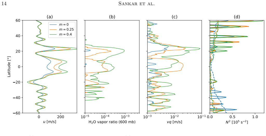
- [Sec. 5.4, Fig. 11] Figure 11(b) shows that the 600 mb vapor ratio is not monotonic in m at all latitudes (e.g., near 45 deg S); the text in Sec. 5.4 states generally that 'the strength of the eddy transport increases with zonal wind shear.' A sentence qualifying this generalization to the latitudes where the mechanism operates would help the reader reconcile panel (b) with the claim.
Circularity Check
No significant circularity in the central CAPE-tendency claim; one minor circular self-consistency check in the cloud-top scaling.
-
fitted input called prediction
[Section 4.1 (Cloud formation); cf. Section 3.1, Eq. 10]
"The equator and 20◦N are also where our methane-band scaling (Fig. 5) defines the highest cloud tops, providing a self-consistent justification for the scaling assumption."
The cloud-top pressure p0 is set from the same Hubble CH4 reflectivity (Section 3.1) and enters the wind profile u(p) via Eq. 10. The model's cloud heights are therefore partly forced by this reflectivity-derived p0, so the coincidence of high modeled clouds at the reflectivity-defined latitudes is a consistency loop rather than an independent justification. The paper itself calls it 'self-consistent,' so it is not a prediction, but the validation uses the same data as the input.
full rationale
The paper's central claim—that the 'chemical' CAPE tendency (eddy water-vapor transport) dominates thermal and mechanical terms—is a diagnostic output, not an input. The three terms in Eq. 9 are evaluated from model state variables using the horizontal-advection tendency of Eq. 12; no parameter is fitted to produce the dominance, and the wind-shear slope m is varied (0, 0.25, 0.4) rather than tuned. The RAS closure (Section 3.2) does set the convective response equal to the total dCAPE/dt by construction, but the decomposition into contributing processes is a posteriori and could in principle have favored thermal or mechanical terms. The no-entrainment simplification in Eq. 9 is explicitly acknowledged in Section 5.1; the cited low-entrainment result (Sankar & Palotai 2022) is a self-citation but is accompanied by a physical rationale and does not by itself force the chemical-term magnitude. A separate correctness risk (not circularity) is that the 'chemical' term includes -L_v dq_sat/dt, which depends on temperature advection through q_sat(T); the paper does not separate this from true vapor advection, so the 'eddy vapor transport' interpretation may overstate the mechanism. The only true circular step is the cloud-top 'self-consistent justification' in Section 4.1, where the CH4-reflectivity input and the model cloud-height output are the same observable. This is minor and does not affect the central diagnostic conclusion.
Assumptions & free parameters
free parameters (7)
- Wind shear slope m =
0, 0.25, 0.4 (0.5 excluded after numerical instability)
- Critical pressure p_c =
30 bar
- Cloud-top pressure p0(latitude) =
scaled from 1 bar to 200 mb from methane-band reflectivity
- RAS relaxation timescale tau_relax =
1 hour
- Bottom heating and top cooling rates =
0.008 W/kg at bottom, 0.01 W/kg at top
- Hyperviscosity coefficients =
nu8, nu_div; nu6 for m=0.4
- Initial perturbation amplitude =
<5 m/s, 100 Gaussian vortices
assumptions (6)
- domain assumption Thermal wind balance relates the 3D temperature field to the zonal wind profile
- ad hoc to paper Convection triggers when CAPE exceeds a critical value, assumed to be zero on Jupiter
- ad hoc to paper The diagnostic parcel does not entrain, so hat(h) = h(z_base)
- ad hoc to paper Tendencies are computed using only horizontal advection (Eq. 12)
- domain assumption The deep wind shear profile (Eq. 10) from Garcia-Melendo et al. (2005) with constant m globally
- domain assumption Eady critical N^2 identifies baroclinic instability regions
Cite this review
Pith. "Pith review of Wind shear and the role of eddy vapor transport in driving water convection on Jupiter." pith.science (2026). https://pith.science/paper/MRLSX5EE
@misc{pith2026250517213,
  author       = {Pith},
  title        = {Pith review of: Wind shear and the role of eddy vapor transport in driving water convection on Jupiter},
  year         = {2026},
  howpublished = {\url{https://pith.science/paper/MRLSX5EE}},
  note         = {Machine review of arXiv:2505.17213}
}
read the original abstract
Recent observations of convection in the jovian atmosphere have demonstrated that convection is strongly concentrated at specific locations on planet. For instance, observations of lightning show that the cyclonic features (e.g,. belts and folded filamentary regions - FFRs) show increased convective activity compared to anti-cyclonic regions. Meanwhile, the distribution of ammonia and water vapor show a large enrichment near the equator, which is also suggestive of strong upwelling and convective activity. Marrying these different observations is challenging due to a lack of data concerning the characteristics of the deep jovian atmosphere, and a resulting inability to observe the true deep source of the various convective phenomena. To understand the nature of these convective events and \paperedit{the role of the } structure of the deep atmosphere \paperedit{in driving convective events}, we run simulations of cloud formation and convection using the Explicit Planetary hybrid-Isentropic Coordinate General Circulation Model (EPIC GCM). We vary the dynamics of the atmosphere by parameterizing the deep wind shear and studying the resulting effect on the strength, frequency and distribution of convective storms. We find that convection in our model is strongly tied to the local dynamics and the deep wind shear. We further decompose the generation of convective available potential energy (CAPE) into three components (thermal, mechanical, and moist/chemical), and find that the chemical mechanism is the strongest component, working to advect water vapor from moisture-rich regions to moisture-poor regions and to drive convection along a ``moisture front.''
Figures


Figures from the paper (13 more)




Reference graph
Works this paper leans on
-
[1]
, " * write output.state after.block = add.period write newline
ENTRY address archivePrefix author booktitle chapter doi edition editor eprint howpublished institution journal key month number organization pages publisher school series title misctitle type volume year version url label extra.label sort.label short.list INTEGERS output.state before.all mid.sentence after.sentence after.block FUNCTION init.state.consts ...
-
[2]
write newline
" write newline "" before.all 'output.state := FUNCTION format.url url empty "" new.block "" url * "" * if FUNCTION format.eprint eprint empty "" archivePrefix empty "" archivePrefix "arXiv" = new.block " " eprint * " " * new.block " " eprint * " " * if if if FUNCTION format.doi doi empty "" " " doi * " " * if FUNCTION format.pid doi empty eprint empty ur...
-
[3]
" id="W5M0MpCehiHzreSzNTczkc9d
thebibliography [1] 20pt to REFERENCES 6pt =0pt \@twocolumntrue 12pt -12pt 10pt plus 3pt =0pt =0pt =1pt plus 1pt =0pt =0pt -12pt =13pt plus 1pt =20pt =13pt plus 1pt \@M =10000 =-1.0em =0pt =0pt 0pt =0pt =1.0em @enumiv\@empty 10000 10000 `\.\@m \@noitemerr \@latex@warning Empty `thebibliography' environment \@ifnextchar \@reference \@latexerr Missing key o...
arXiv 2017
-
[4]
1989, Geochimica et Cosmochimica Acta, 53, 197, https://doi.org/10.1016/0016-7037(89)90286-X
Anders, E., & Grevesse, N. 1989, Geochimica et Cosmochimica Acta, 53, 197, https://doi.org/10.1016/0016-7037(89)90286-X
-
[5]
Arakawa , A., Jung , J. H., & Wu , C. M. 2011, Atmospheric Chemistry & Physics, 11, 3731, 10.5194/acp-11-3731-2011
-
[6]
Arakawa , A., & Schubert , W. H. 1974, Journal of Atmospheric Sciences, 31, 674, 10.1175/1520-0469(1974)031<0674:IOACCE>2.0.CO;2
-
[7]
Asplund , M., Grevesse , N., Sauval , A. J., & Scott , P. 2009, Annual Review of Astronomy and Astrophysics, 47, 481, 10.1146/annurev.astro.46.060407.145222
arXiv 2009
-
[8]
Atkinson , D. H., Pollack , J. B., & Seiff , A. 1998, Journal of Geophysical Research, 103, 22911, 10.1029/98JE00060
Show all 76 references
-
[9]
L., Wong , M
Bjoraker , G. L., Wong , M. H., de Pater , I., Hewagama , T., & \'A d \'a mkovics , M. 2022, Remote Sensing, 14, 4567, 10.3390/rs14184567
2022 doi
-
[10]
2024, , 687, A274, 10.1051/0004-6361/202245220
Boissinot , A., Spiga , A., Guerlet , S., Cabanes , S., & Bardet , D. 2024, , 687, A274, 10.1051/0004-6361/202245220
2024 doi
-
[11]
2018, , 558, 87, 10.1038/s41586-018-0156-5
Brown , S., Janssen , M., Adumitroaie , V., et al. 2018, , 558, 87, 10.1038/s41586-018-0156-5
2018 doi
-
[12]
R., Zhang, Z., Rogers, J
Brueshaber, S. R., Zhang, Z., Rogers, J. H., et al. 2025, , 116465, https://doi.org/10.1016/j.icarus.2025.116465
2025
-
[13]
S., et al
Cao , H., Bloxham , J., Park , R. S., et al. 2023, , 959, 78, 10.3847/1538-4357/ad0cbb
2023 doi
-
[14]
M., & Moeckel , C
de Pater , I., Molter , E. M., & Moeckel , C. M. 2023, Remote Sensing, 15, 1313, 10.3390/rs15051313
2023 doi
-
[16]
2019 b , The Astronomical Journal, 158, 139, 10.3847/1538-3881/ab3643
---. 2019 b , The Astronomical Journal, 158, 139, 10.3847/1538-3881/ab3643
2019 doi
-
[17]
E., Fischer , A
Dowling , T. E., Fischer , A. S., Gierasch , P. J., et al. 1998, , 132, 221, 10.1006/icar.1998.5917
1998
-
[18]
E., & Gierasch , P
Dowling , T. E., & Gierasch , P. J. 1989, in Bulletin of the American Astronomical Society, Vol. 21, 946
1989
-
[19]
E., Bradley , M
Dowling , T. E., Bradley , M. E., Col \'o n , E., et al. 2006, , 182, 259, 10.1016/j.icarus.2006.01.003
2006 doi
-
[20]
2021, arXiv e-prints, arXiv:2110.07255
Duer , K., Gavriel , N., Galanti , E., et al. 2021, arXiv e-prints, arXiv:2110.07255. 2110.07255
2021 arXiv
-
[21]
A., Del Genio , A
Dyudina , U. A., Del Genio , A. D., Ingersoll , A. P., et al. 2004, , 172, 24, 10.1016/j.icarus.2004.07.014
2004 doi
-
[22]
M., Kunde , V
Flasar , F. M., Kunde , V. G., Achterberg , R. K., et al. 2004, , 427, 132, 10.1038/nature02142
2004 doi
-
[23]
N., Orton , G
Fletcher , L. N., Orton , G. S., Rogers , J. H., et al. 2017, , 286, 94, 10.1016/j.icarus.2017.01.001
2017 doi
-
[24]
N., Orton , G
Fletcher , L. N., Orton , G. S., Greathouse , T. K., et al. 2020, Journal of Geophysical Research (Planets), 125, e06399, 10.1029/2020JE006399
2020 doi
-
[25]
N., Oyafuso , F
Fletcher , L. N., Oyafuso , F. A., Allison , M., et al. 2021, Journal of Geophysical Research (Planets), 126, e06858, 10.1029/2021JE006858
2021 doi
-
[26]
Garc \' a-Melendo , E., S \'a nchez-Lavega , A., & Dowling , T. E. 2005, , 176, 272, 10.1016/j.icarus.2005.02.012
2005 doi
-
[27]
2024, , 5, 101, 10.3847/PSJ/ad0ed3
Ge , H., Li , C., Zhang , X., & Moeckel , C. 2024, , 5, 101, 10.3847/PSJ/ad0ed3
2024 doi
-
[28]
J., Conrath , B
Gierasch , P. J., Conrath , B. J., & Magalh \ a es , J. A. 1986, , 67, 456, 10.1016/0019-1035(86)90125-9
1986 doi
-
[29]
J., Ingersoll , A
Gierasch , P. J., Ingersoll , A. P., Banfield , D., et al. 2000, , 403, 628, 10.1038/35001017
2000 doi
-
[30]
S., Greathouse , T
Giles , R. S., Greathouse , T. K., Bonfond , B., et al. 2020, Journal of Geophysical Research (Planets), 125, e06659, 10.1029/2020JE006659
2020 doi
-
[31]
Grevesse, N., & Sauval, A. J. 2001, Solar Abundances, ed. P. Murdin (Boca Raton, FL: CRC Press / Taylor & Francis Group), 4088--4091, 10.1201/9781003220435
2001 doi
-
[32]
1995, Science, 269, 1697, 10.1126/science.7569896
Guillot , T. 1995, Science, 269, 1697, 10.1126/science.7569896
1995 doi
-
[33]
J., et al
Guillot , T., Li , C., Bolton , S. J., et al. 2020, Journal of Geophysical Research (Planets), 125, e06404, 10.1029/2020JE006404
2020 doi
-
[34]
Holton, J. R. 2004, An introduction to dynamic meteorology , 4th edn., ed. R. Dmowska & J. R. Holton, International Geophysics Series (Burlington, MA: Elsevier Academic Press,), 535. http://books.google.com/books?id=fhW5oDv3EPsC
2004
-
[35]
2001, , 151, 257, 10.1006/icar.2000.6606
Hueso , R., & S \'a nchez-Lavega , A. 2001, , 151, 257, 10.1006/icar.2000.6606
2001
-
[36]
2022, , 380, 114994, 10.1016/j.icarus.2022.114994
Hueso , R., I \ n urrigarro , P., S \'a nchez-Lavega , A., et al. 2022, , 380, 114994, 10.1016/j.icarus.2022.114994
2022
-
[37]
2020, , 336, 113475, 10.1016/j.icarus.2019.113475
I \ n urrigarro , P., Hueso , R., Legarreta , J., et al. 2020, , 336, 113475, 10.1016/j.icarus.2019.113475
2020
-
[38]
H., Kolma s ov \'a , I., et al
Imai , M., Wong , M. H., Kolma s ov \'a , I., et al. 2020, Geophysical Research Letters, 47, e88397, 10.1029/2020GL088397
2020 doi
-
[39]
P., Gierasch , P
Ingersoll , A. P., Gierasch , P. J., Banfield , D., Vasavada , A. R., & Galileo Imaging Team . 2000, , 403, 630, 10.1038/35001021
2000 doi
-
[40]
2018, Nature Astronomy, 2, 544, 10.1038/s41550-018-0442-z
Kolma s ov \'a , I., Imai , M., Santol \' k , O., et al. 2018, Nature Astronomy, 2, 544, 10.1038/s41550-018-0442-z
2018 doi
-
[41]
2017, , 598, A98, 10.1051/0004-6361/201629140
Leconte , J., Selsis , F., Hersant , F., & Guillot , T. 2017, , 598, A98, 10.1051/0004-6361/201629140
2017 doi
-
[42]
2019, , 240, 37, 10.3847/1538-4365/aafdaa
Li , C., & Chen , X. 2019, , 240, 37, 10.3847/1538-4365/aafdaa
2019 doi
-
[43]
Li , C., & Ingersoll , A. P. 2015, Nature Geoscience, 8, 398, 10.1038/ngeo2405
2015 doi
-
[44]
2017, , 44, 5317, 10.1002/2017GL073159
Li , C., Ingersoll , A., Janssen , M., et al. 2017, , 44, 5317, 10.1002/2017GL073159
2017 doi
-
[45]
2020, Nature Astronomy, 4, 609, 10.1038/s41550-020-1009-3
Li , C., Ingersoll , A., Bolton , S., et al. 2020, Nature Astronomy, 4, 609, 10.1038/s41550-020-1009-3
2020 doi
-
[46]
2024, Icarus, 414, 116028, 10.1016/j.icarus.2024.116028
Li , C., Allison , M., Atreya , S., et al. 2024, Icarus, 414, 116028, 10.1016/j.icarus.2024.116028
2024
-
[47]
A., et al
Li , L., Jiang , X., West , R. A., et al. 2018, Nature Communications, 9, 3709, 10.1038/s41467-018-06107-2
2018 doi
-
[48]
Lian , Y., & Showman , A. P. 2010, , 207, 373, 10.1016/j.icarus.2009.10.006
2010 doi
-
[49]
D., Ingersoll , A
Little , B., Anger , C. D., Ingersoll , A. P., et al. 1999, Icarus, 142, 306, 10.1006/icar.1999.6195
1999
-
[50]
2010, in Astrophysics and Space Science Proceedings, Vol
Lodders , K. 2010, in Astrophysics and Space Science Proceedings, Vol. 16, Principles and Perspectives in Cosmochemistry, ed. A. Goswami & B. E. Reddy , 379, 10.1007/978-3-642-10352-0_8
2010 doi
-
[51]
2021, Space Science Reviews, 217, 44, 10.1007/s11214-021-00825-8
Lodders , K. 2021, Space Science Reviews, 217, 44, 10.1007/s11214-021-00825-8
2021 doi
-
[52]
R., Macgorman , D
Mansell , E. R., Macgorman , D. R., Ziegler , C. L., & Straka , J. M. 2005, Journal of Geophysical Research (Atmospheres), 110, D12101, 10.1029/2004JD005287
2005 doi
-
[53]
2023, , 4, 25, 10.3847/PSJ/acaf6b
Moeckel , C., de Pater , I., & DeBoer , D. 2023, , 4, 25, 10.3847/PSJ/acaf6b
2023 doi
-
[54]
Moorthi , S., & Suarez , M. J. 1992, Monthly Weather Review, 120, 978, 10.1175/1520-0493(1992)120<0978:RASAPO>2.0.CO;2
1992 doi
-
[55]
Moorthi, S., & Suarez, M. J. 1999, NOAA technical report NWS/NCEP. https://repository.library.noaa.gov/view/noaa/11400
1999
-
[56]
I., Fouchet , T., Bezard , B., et al
Moses , J. I., Fouchet , T., Bezard , B., et al. 2005, Journal of Geophysical Research (Planets), 110, E08001, 10.1029/2005JE002411
2005 doi
-
[57]
B., Atreya , S
Niemann , H. B., Atreya , S. K., Carignan , G. R., et al. 1998, Journal of Geophysical Research, 103, 22831, 10.1029/98JE01050
1998 doi
-
[58]
S., Momary , T., Ingersoll , A
Orton , G. S., Momary , T., Ingersoll , A. P., et al. 2017, Geophysical Research Letters, 44, 4607, 10.1002/2017GL073019
2017 doi
-
[59]
2022, Remote Sensing, 15, 219, 10.3390/rs15010219
Palotai , C., Brueshaber , S., Sankar , R., & Sayanagi , K. 2022, Remote Sensing, 15, 219, 10.3390/rs15010219
2022 doi
-
[60]
Palotai , C., & Dowling , T. E. 2008, , 194, 303, 10.1016/j.icarus.2007.10.025
2008 doi
-
[61]
M., Moore, J
Rochette, S. M., Moore, J. T., & Market, P. S. 1999, Natl. Wea. Dig, 23, 20
1999
-
[62]
2021, , 368, 114589, 10.1016/j.icarus.2021.114589
Sankar , R., Klare , C., & Palotai , C. 2021, , 368, 114589, 10.1016/j.icarus.2021.114589
2021
-
[63]
2022, , 380, 114973, 10.1016/j.icarus.2022.114973
Sankar , R., & Palotai , C. 2022, , 380, 114973, 10.1016/j.icarus.2022.114973
2022
-
[64]
Showman , A. P. 2007, Journal of Atmospheric Sciences, 64, 3132, 10.1175/JAS4007.1
2007 doi
-
[65]
A., Wong , M
Simon , A. A., Wong , M. H., & Orton , G. S. 2015, The Astrophysical Journal, 812, 55, 10.1088/0004-637X/812/1/55
2015 doi
-
[66]
A., Soderblom , L
Smith , B. A., Soderblom , L. A., Johnson , T. V., et al. 1979, Science, 204, 951, 10.1126/science.204.4396.951
1979 doi
-
[67]
Sugiyama , K., Nakajima , K., Odaka , M., Kuramoto , K., & Hayashi , Y. Y. 2014, , 229, 71, 10.1016/j.icarus.2013.10.016
2014 doi
-
[68]
H., Pater , I
Tollefson , J., Wong , M. H., Pater , I. d., et al. 2017, , 296, 163, 10.1016/j.icarus.2017.06.007
2017 doi
-
[69]
Vallis , G. K. 2017, Atmospheric and Oceanic Fluid Dynamics: Fundamentals and Large-Scale Circulation , 10.1017/9781107588417
2017 doi
-
[70]
R., & Showman , A
Vasavada , A. R., & Showman , A. P. 2005, Reports on Progress in Physics, 68, 1935, 10.1088/0034-4885/68/8/R06
2005 doi
-
[71]
2017, Dataset: Wide Field Coverage for Juno (WFCJ), MAST archive at Space Telescope Science Institute, 10.17909/T94T1H
Wong, M. 2017, Dataset: Wide Field Coverage for Juno (WFCJ), MAST archive at Space Telescope Science Institute, 10.17909/T94T1H
2017 doi
-
[72]
H., Atreya , S
Wong , M. H., Atreya , S. K., Kuhn , W. R., Romani , P. N., & Mihalka , K. M. 2015, , 245, 273, 10.1016/j.icarus.2014.09.042
2015 doi
-
[73]
H., Bjoraker , G
Wong , M. H., Bjoraker , G. L., Goullaud , C., et al. 2023, Remote Sensing, 15, 702, 10.3390/rs15030702
2023 doi
-
[74]
H., Mahaffy, P
Wong, M. H., Mahaffy, P. R., Atreya, S. K., Niemann, H. B., & Owen, T. C. 2004, Icarus, 171, 153
2004
-
[75]
H., Simon , A
Wong , M. H., Simon , A. A., Tollefson , J. W., et al. 2020, , 247, 58, 10.3847/1538-4365/ab775f
2020 doi
-
[76]
Young , R. M. B., Read , P. L., & Wang , Y. 2019 a , , 326, 225, 10.1016/j.icarus.2018.12.005
2019 doi
-
[77]
2019 b , , 326, 253, 10.1016/j.icarus.2018.12.002
---. 2019 b , , 326, 253, 10.1016/j.icarus.2018.12.002
2019 doi
Reviewed August 7, 2026 · model on record in the stance chip above.
Discussion (0). Continue with ORCID to comment.