REVIEW 3 major objections 4 minor 95 references
Search for the nonresonant and resonant production of a Higgs boson in association with an additional scalar boson in the $\gamma\gamma\tau\tau$ final state in proton-proton collisions at $\sqrt{s}$ = 13 TeV
T0 review · 3 major / 4 minor · reviewed 2026-08-06 · deepseek-v4-flash
Pith's one-line read A search in γγττ final states finds no evidence for pair production of scalar bosons and sets the tightest limits yet from this channel on the Higgs trilinear self-coupling.
desk verdict First γγττ HH/X→HH/X→YH search from CMS, no signal, solid limits; the background-envelope closure is the only caveat worth arguing about. read the letter →
The pith
A machine-rendered reading of the paper's core claim, the machinery that carries it, and where it could break.
The reading
What carries the argument
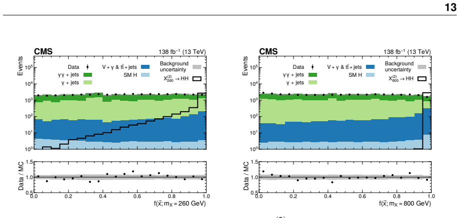
The analysis extracts results from simultaneous maximum-likelihood fits to the diphoton invariant mass mγγ in event categories defined by machine-learning classifiers: a boosted decision tree for the nonresonant search and parameterized neural networks (pNNs) for the resonant searches, where the nominal masses mX and mY are fed to the network as input features so one classifier interpolates across mass hypotheses. The continuum background is modeled directly from data using the discrete profiling method, which treats the choice of analytic function (exponentials, Bernstein polynomials, Laurent series, power laws) as a discrete nuisance parameter and thereby accounts for the systematic uncertainty in the background shape. Signal shapes are modeled with double Crystal Ball functions fitted to simulation.
What would settle it
Apply the BDT and pNN selections to a background-only control sample, such as simulated γ+jets events, and inspect the resulting mγγ spectrum for a visible peak near 125 GeV; a peak would indicate selection-induced sculpting and bias the fitted limits. A complementary check is to repeat the full fit with a broader family of background functions and see whether the best-fit signal strength or the κλ exclusion interval shifts by more than the quoted systematic uncertainty.
Extended reading notes
Core claim
The analysis reports that, in the diphoton-plus-two-tau final state, the data are consistent with background-only expectations. For nonresonant HH production the observed (expected) 95% CL upper limit on the cross section is 930 (740) fb, corresponding to 33 (26) times the standard-model prediction, and HH production is excluded for κλ outside the observed (expected) range between −12 (−9.4) and 17 (15). For resonant X→HH production, observed (expected) limits on σ(pp→X)B(X→HH) lie between 160 and 2200 (200 and 1800) fb depending on the mass of X. The X→YH searches set observed (expected) upper limits on σ(pp→X)B(X→YH→γγττ) between 0.059 and 1.2 fb (0.087 and 0.68 fb) for the Y→ττ channel, and between 0.69 and 15 fb (0.73 and 8.3 fb) for the low-mass Y→γγ channel, where a region of the NMSSM parameter space is more tightly constrained than before. The largest local excesses have significances of 2.6–3.2σ, but their global significances are 0.1–2.2σ, so no standalone evidence for new physics is claimed.
Load-bearing premise
The continuum diphoton background is smoothly falling and correctly described by the family of analytic functions chosen by the discrete profiling method in every analysis category, and the machine-learning selections do not sculpt peaking structure in the mγγ distribution.
Editorial extensions
If this is right
- If the central claim is correct, HH production at 13 TeV is at most about 33 times the standard-model rate, providing a direct upper bound on the Higgs trilinear self-coupling.
- The κλ constraint excludes HH production for self-coupling modifiers outside the interval from −12 to 17, assuming all other Higgs couplings are standard-model-like.
- The resonant X→HH limits constrain spin-0 and spin-2 resonances, excluding, for example, certain bulk radion and Kaluza–Klein graviton masses in the Randall–Sundrum model.
- The X→YH limits reach cross sections below 1 fb in the low Y-mass regime, tightening the allowed NMSSM parameter space in a region of (mX, mY).
- The local excesses near mY ≈ 95 GeV, while globally insignificant, are consistent with other CMS excesses and motivate dedicated future measurements at those masses.
Reading between the lines
- Combining this γγττ search with other HH channels, such as bbγγ and ττ final states, could tighten the κλ interval further than any single channel alone.
- The parameterized neural-network approach used here is a reusable template for future resonance searches that need to interpolate signal models over a two-dimensional mass plane.
- The recurring excess near 95 GeV across independent final states hints at a possible light scalar that the present search cannot confirm but that the next LHC data-taking period could settle.
- The published σ×B limits can be reinterpreted in other beyond-standard-model frameworks beyond the RS and NMSSM examples shown in the paper.
Editorial analysis
A structured set of objections, weighed in public.
Referee Report
Summary. This CMS paper presents a search for nonresonant Higgs-pair production and for resonant production of two scalars in the γγττ final state, using up to 138 fb^-1 of 13 TeV pp collision data. Five searches are performed: nonresonant ggF HH, spin-0 and spin-2 X→HH, X→Y(ττ)H(γγ), and low- and high-mass X→Y(γγ)H(ττ). Events are categorized with a BDT (nonresonant) or parameterized neural networks (resonant), and limits are extracted from fits to the diphoton invariant mass using the discrete profiling method for the continuum background. No significant excess is found. The observed (expected) 95% CL upper limit on nonresonant HH production is 930 (740) fb, i.e., 33 (26) times the SM prediction, and κλ is constrained to lie between -12 and 17. Resonant X→HH limits range from 160 to 2200 fb, while the X→YH searches set limits on σB that reach below 0.1 fb in the most sensitive regions. Tabulated results are provided in HEPData.
Significance. The search is competently executed and covers a broad set of final states and mass hypotheses. Its main value is in constraining BSM scalar production in the γγττ channel, particularly the X→YH topologies, where the low-mass Y→γγ search places limits below the maximally allowed NMSSM cross sections in a region of (mX, mY). The nonresonant HH limit is not competitive with the combined CMS/ATLAS results, but the κλ scan and the thirteen EFT benchmark limits provide useful input to global HH interpretations. Strengths of the paper include the use of pseudo-experiments where the asymptotic approximation fails, explicit treatment of background-function uncertainty with the discrete profiling method, validation of the pNN interpolation between mass points, and the public HEPData record. The main weakness is the limited validation of the background-model envelope against out-of-family shapes and the somewhat large accepted residual bias in the significance calculation.
major comments (3)
- [§7, §8.3] The residual-bias checks described in §7 and §8.3 validate the discrete profiling method only against pseudo-datasets generated from functions that belong to the same candidate family set used in the envelope. This does not directly probe out-of-family background shapes, such as smooth threshold effects, trigger turn-on residuals, or two-component mixtures with energy-dependent slopes. Because the reported upper limits and the κλ exclusion range are extracted from fits in which the continuum shape is entirely data-driven, an out-of-family closure test—for example, generating pseudo-datasets from smooth functions outside the candidate families and checking the bias on the fitted signal yield—would directly support the claim that the background-function choice contributes negligibly to the limits. The <1% systematic impact quoted in §9 refers to the fitted nuisance parameters and does not by itself address this coverage question.
- [§7] The paper states that a minimum of 10 expected background events per category was chosen because it 'still led to acceptable bias of 20%' in the significance. A 20% bias in significances is large, and the manuscript does not reconcile this with §9's statement that the combined impact of all systematic uncertainties is less than 1% on the upper limits. Please quantify the corresponding bias on the final 95% CL upper limits (not on significances) for the categories with 10 expected events, or explicitly propagate a conservative form of this residual bias into the quoted limits.
- [§10.1] The κλ result neglects the κλ-dependent NLO electroweak corrections to single-H production, as noted in the text after Fig. 9. Since single-H production contributes a resonant background at the same mass as the HH signal and the κλ interpretation is based on the signal-strength dependence, a quantitative estimate or a clear argument for the negligible impact of this correction is needed before the quoted κλ interval can be considered robust.
minor comments (4)
- [Fig. 12 caption] The caption contains a duplicated phrase: 'as a function as a function of mY'; please correct.
- [§5] There is a typo in 'psudorapidity'; it should be 'pseudorapidity'.
- [§9] The phrase 'nonresonant background estimation' appears to mean 'continuum background estimation'; please clarify to avoid confusion with the nonresonant HH search.
- [§8.2] The interpolation uncertainty for intermediate mass points is evaluated by removing the nearest nominal mass point. This is reasonable, but it may underestimate nonlinearities in the efficiency or shape; a brief comment on the expected size of this effect would be helpful.
Circularity Check
No significant circularity: the reported limits are extracted from data fits with external inputs, and no fitted parameter is recycled as a prediction.
full rationale
The central numerical claims—the 930 fb upper limit on HH production, the kappa-lambda exclusion range between -12 and 17, and the resonant limits—are obtained from maximum likelihood fits to the observed diphoton mass distributions. The continuum background is modeled directly from data using the discrete profiling method over an ensemble of analytic functions, with sidebands used where appropriate (Section 8.3); the signal and single-Higgs resonant background shapes and normalizations come from simulation and from external LHC Higgs working group inputs (Ref. [15]), not from fitted parameters of this analysis. Expected limits are derived from background-only simulation, so no fitted value is renamed or reused as a prediction. The residual-bias closure test described in Section 7, in which pseudo-datasets are generated from one of the candidate background functions and the significance is compared with the background function fixed or floating, is explicitly a check of bias within the chosen function envelope; the text does not claim it validates background shapes outside that family, and the final limits do not reduce to that test. Citations to earlier CMS searches are motivational only and are not load-bearing for the limit-setting derivation. There is no self-definitional step, no fitted input called a prediction, and no imported uniqueness theorem. The analysis is therefore self-contained against external benchmarks and exhibits no significant circularity.
Assumptions & free parameters
assumptions (5)
- domain assumption The m_gamma_gamma continuum background is smoothly falling and can be represented by one member of the candidate function families used in the discrete profiling method.
- domain assumption Simulated events reproduce the CMS detector response, trigger, and object efficiencies after data-to-simulation corrections.
- domain assumption The new particles X and Y have narrow width compared to the experimental mass resolution.
- ad hoc to paper Signal efficiencies and shape parameters interpolate smoothly between generated mass points via linear or cubic splines.
- domain assumption The external standard model inputs (m_H = 125.38 GeV, branching fractions, and HH cross section predictions) are correct and applicable.
Cite this review
Pith. "Pith review of Search for the nonresonant and resonant production of a Higgs boson in association with an additional scalar boson in the $\gamma\gamma\tau\tau$ final state in proton-proton collisions at $\sqrt{s}$ = 13 TeV." pith.science (2026). https://pith.science/paper/NWTWORHS
@misc{pith2026250623012,
  author       = {Pith},
  title        = {Pith review of: Search for the nonresonant and resonant production of a Higgs boson in association with an additional scalar boson in the $\gamma\gamma\tau\tau$ final state in proton-proton collisions at $\sqrts$ = 13 TeV},
  year         = {2026},
  howpublished = {\url{https://pith.science/paper/NWTWORHS}},
  note         = {Machine review of arXiv:2506.23012}
}
abstract
The results of a search for the production of two scalar bosons in final states with two photons and two tau leptons are presented. The search considers both nonresonant production of a Higgs boson pair, HH, and resonant production via a new boson X which decays either to HH or to H and a new scalar Y. The analysis uses up to 138 fb$^{-1}$ of proton-proton collision data, recorded between 2016 and 2018 by the CMS experiment at the LHC at a center-of-mass energy of 13 TeV. No evidence for signal is found in the data. For the nonresonant production, the observed (expected) upper limit at 95% confidence level (CL) on the HH production cross section is set at 930 (740) fb, corresponding to 33 (26) times the standard model prediction. At 95% CL, HH production is observed (expected) to be excluded for values of $\kappa_\lambda$ outside the range between $-$12 ($-$9.4) and 17 (15). Observed (expected) upper limits at 95% CL for the X $\to$ HH cross section are found to be within 160 to 2200 (200 to 1800) fb, depending on the mass of X. In the X $\to$ Y($\tau\tau$)H($\gamma\gamma$) search, the observed (expected) upper limits on the product of the production cross section and decay branching fractions vary between 0.059$-$1.2 fb (0.087$-$0.68 fb). For the X $\to$ Y($\gamma\gamma$)H($\tau\tau$) search the observed (expected) upper limits on the product of the production cross section and Y $\to$ $\gamma\gamma$ branching fraction vary between 0.69$-$15 fb (0.73$-$8.3 fb) in the low Y mass search, tightening constraints on the next-to-minimal supersymmetric standard model, and between 0.64$-$10 fb (0.70$-$7.6 fb) in the high Y mass search.
Figures


Figures from the paper (19 more)


Reference graph
Works this paper leans on
-
[1]
ATLAS Collaboration, “Observation of a new particle in the search for the standard model Higgs boson with the atlas detector at the LHC”,Phys. Lett. B716(2012) 1, doi:10.1016/j.physletb.2012.08.020,arXiv:1207.7214
arXiv 2012
-
[2]
Observation of a new boson at a mass of 125 GeV with the CMS experiment at the LHC
CMS Collaboration, “Observation of a new boson at a mass of 125 GeV with the CMS experiment at the LHC”,Phys. Lett. B716(2012) 30, doi:10.1016/j.physletb.2012.08.021,arXiv:1207.7235
arXiv 2012
-
[3]
Observation of a new boson with mass near 125 GeV in pp collisions at √s= 7 and 8 TeV
CMS Collaboration, “Observation of a new boson with mass near 125 GeV in pp collisions at √s= 7 and 8 TeV”,JHEP06(2013) 081, doi:10.1007/JHEP06(2013)081,arXiv:1303.4571. References 37
arXiv 2013
-
[4]
A portrait of the Higgs boson by the CMS experiment ten years after the discovery
CMS Collaboration, “A portrait of the Higgs boson by the CMS experiment ten years after the discovery”,Nature607(2022) 60,doi:10.1038/s41586-022-04892-x, arXiv:2207.00043
arXiv 2022
-
[5]
A detailed map of Higgs boson interactions by the ATLAS experiment ten years after the discovery
ATLAS Collaboration, “A detailed map of Higgs boson interactions by the ATLAS experiment ten years after the discovery”,Nature607(2022) 52, doi:10.1038/s41586-022-04893-w,arXiv:2207.00092. [Erratum: doi:10.1038/s41586-022-05581-5]
arXiv 2022
-
[6]
Higgs boson pair production at NNLO with top quark mass effects
M. Grazzini et al., “Higgs boson pair production at NNLO with top quark mass effects”, JHEP05(2018) 059,doi:10.1007/JHEP05(2018)059,arXiv:1803.02463
arXiv 2018
-
[7]
Neutral Higgs boson pair production at hadron colliders: QCD corrections
S. Dawson, S. Dittmaier, and M. Spira, “Neutral Higgs boson pair production at hadron colliders: QCD corrections”,Phys. Rev. D58(1998) 115012, doi:10.1103/PhysRevD.58.115012,arXiv:hep-ph/9805244
arXiv 1998
-
[8]
S. Borowka et al., “Higgs boson pair production in gluon fusion at next-to-leading order with full top-quark mass dependence”,Phys. Rev. Lett.117(2016) 012001, doi:10.1103/PhysRevLett.117.079901,arXiv:1604.06447. [Erratum: doi:10.1103/PhysRevLett.117.079901]
arXiv 2016
Show all 95 references
-
[9]
Gluon fusion into Higgs pairs at NLO QCD and the top mass scheme
J. Baglio et al., “Gluon fusion into Higgs pairs at NLO QCD and the top mass scheme”, Eur. Phys. J. C79(2019) 459,doi:10.1140/epjc/s10052-019-6973-3, arXiv:1811.05692
2019 arXiv
-
[10]
Higgs boson pair production at next-to-next-to-leading order in QCD
D. de Florian and J. Mazzitelli, “Higgs boson pair production at next-to-next-to-leading order in QCD”,Phys. Rev. Lett.111(2013) 201801, doi:10.1103/PhysRevLett.111.201801,arXiv:1309.6594
2013 arXiv
-
[11]
Threshold resummation effects in Higgs boson pair production at the LHC
D. Y. Shao, C. S. Li, H. T. Li, and J. Wang, “Threshold resummation effects in Higgs boson pair production at the LHC”,JHEP07(2013) 169,doi:10.1007/JHEP07(2013)169, arXiv:1301.1245
2013 arXiv
-
[12]
Higgs pair production at next-to-next-to-leading logarithmic accuracy at the LHC
D. de Florian and J. Mazzitelli, “Higgs pair production at next-to-next-to-leading logarithmic accuracy at the LHC”,JHEP09(2015) 053, doi:10.1007/JHEP09(2015)053,arXiv:1505.07122
2015 arXiv
-
[13]
gg→hh: Combined uncertainties
J. Baglio et al., “gg→hh: Combined uncertainties”,Phys. Rev. D103(2021) 056002, doi:10.1103/PhysRevD.103.056002,arXiv:2008.11626
2021 arXiv
-
[14]
Constraints on the Higgs boson self-coupling from single- and double-Higgs production with the ATLAS detector using pp collisions at s=13 TeV
ATLAS Collaboration, “Constraints on the Higgs boson self-coupling from single- and double-Higgs production with the ATLAS detector using pp collisions at s=13 TeV”, Phys. Lett. B843(2023) 137745,doi:10.1016/j.physletb.2023.137745, arXiv:2211.01216
2023
-
[15]
Handbook of LHC Higgs cross sections: 4. Deciphering the nature of the Higgs sector
LHC Higgs Cross Section Working Group, “Handbook of LHC Higgs cross sections: 4. Deciphering the nature of the Higgs sector”, CERN Report CERN-2017-002-M, 2016. doi:10.23731/CYRM-2017-002,arXiv:1610.07922
2017 arXiv
-
[16]
Higgs boson pair production in the D=6 extension of the SM
F. Goertz, A. Papaefstathiou, L. L. Yang, and J. Zurita, “Higgs boson pair production in the D=6 extension of the SM”,JHEP04(2015) 167,doi:10.1007/JHEP04(2015)167, arXiv:1410.3471. 38
2015 arXiv
-
[17]
A large mass hierarchy from a small extra dimension
L. Randall and R. Sundrum, “A large mass hierarchy from a small extra dimension”, Phys. Rev. Lett.83(1999) 3370,doi:10.1103/PhysRevLett.83.3370, arXiv:hep-ph/9905221
1999 arXiv
-
[18]
Modulus stabilization with bulk fields
W. D. Goldberger and M. B. Wise, “Modulus stabilization with bulk fields”,Phys. Rev. Lett.83(1999) 4922,doi:10.1103/PhysRevLett.83.4922, arXiv:hep-ph/9907447
1999 arXiv
-
[19]
Phenomenology of the Randall-Sundrum gauge hierarchy model
H. Davoudiasl, J. L. Hewett, and T. G. Rizzo, “Phenomenology of the Randall-Sundrum gauge hierarchy model”,Phys. Rev. Lett.84(2000) 2080, doi:10.1103/PhysRevLett.84.2080,arXiv:hep-ph/9909255
2000 arXiv
-
[20]
The anatomy of electro-weak symmetry breaking. II. the Higgs bosons in the minimal supersymmetric model
A. Djouadi, “The anatomy of electro-weak symmetry breaking. II. the Higgs bosons in the minimal supersymmetric model”,Phys. Rept.459(2008) 1, doi:10.1016/j.physrep.2007.10.005,arXiv:hep-ph/0503173
2008 arXiv
-
[21]
Search for a new resonance decaying into two spin-0 bosons in a final state with two photons and two bottom quarks in proton-proton collisions at √s= 13 TeV
CMS Collaboration, “Search for a new resonance decaying into two spin-0 bosons in a final state with two photons and two bottom quarks in proton-proton collisions at √s= 13 TeV”,JHEP05(2024) 316,doi:10.1007/JHEP05(2024)316, arXiv:2310.01643
2024 arXiv
-
[22]
Searches for additional Higgs bosons and for vector leptoquarks in ττfinal states in proton-proton collisions at √s= 13 TeV
CMS Collaboration, “Searches for additional Higgs bosons and for vector leptoquarks in ττfinal states in proton-proton collisions at √s= 13 TeV”,JHEP07(2023) 073, doi:10.1007/JHEP07(2023)073,arXiv:2208.02717
2023 arXiv
-
[23]
Search for a standard model-like Higgs boson in the mass range between 70 and 110 GeV in the diphoton final state in proton-proton collisions at √s= 13 TeV
CMS Collaboration, “Search for a standard model-like Higgs boson in the mass range between 70 and 110 GeV in the diphoton final state in proton-proton collisions at √s= 13 TeV”,Phys. Lett. B860(2025) 139067,doi:10.1016/j.physletb.2024.139067, arXiv:2405.18149
2025
-
[24]
Higgs pair production: Choosing benchmarks with cluster analysis
A. Carvalho et al., “Higgs pair production: Choosing benchmarks with cluster analysis”, JHEP04(2016) 126,doi:10.1007/JHEP04(2016)126,arXiv:1507.02245
2016 arXiv
-
[25]
Higgs boson pair production in non-linear effective field theory with fullm t-dependence at NLO QCD
G. Buchalla et al., “Higgs boson pair production in non-linear effective field theory with fullm t-dependence at NLO QCD”,JHEP09(2018) 057, doi:10.1007/JHEP09(2018)057,arXiv:1806.05162
2018 arXiv
-
[26]
HEPData record for this analysis
“HEPData record for this analysis”, 2025.doi:10.17182/hepdata.158371
2025 doi
-
[27]
The CMS experiment at the CERN LHC
CMS Collaboration, “The CMS experiment at the CERN LHC”,JINST3(2008) S08004, doi:10.1088/1748-0221/3/08/S08004
2008 doi
-
[28]
Performance of the CMS level-1 trigger in proton-proton collisions at √s=13 TeV
CMS Collaboration, “Performance of the CMS level-1 trigger in proton-proton collisions at √s=13 TeV”,JINST15(2020) P10017, doi:10.1088/1748-0221/15/10/P10017,arXiv:2006.10165
2020 arXiv
-
[29]
The CMS trigger system
CMS Collaboration, “The CMS trigger system”,JINST12(2017) P01020, doi:10.1088/1748-0221/12/01/P01020,arXiv:1609.02366
2017 arXiv
-
[30]
Performance of the CMS high-level trigger during LHC run 2
CMS Collaboration, “Performance of the CMS high-level trigger during LHC run 2”, JINST19(2024) P11021,doi:10.1088/1748-0221/19/11/P11021, arXiv:2410.17038. References 39
2024 arXiv
-
[31]
Particle-flow reconstruction and global event description with the CMS detector
CMS Collaboration, “Particle-flow reconstruction and global event description with the CMS detector”,JINST12(2017) P10003,doi:10.1088/1748-0221/12/10/P10003, arXiv:1706.04965
2017 arXiv
-
[32]
Technical proposal for the Phase-II upgrade of the CMS detector
D. Contardo et al., “Technical proposal for the Phase-II upgrade of the CMS detector”, technical report, Geneva, 2015.doi:10.17181/CERN.VU8I.D59J
2015 doi
-
[33]
Electron and photon reconstruction and identification with the CMS experiment at the CERN LHC
CMS Collaboration, “Electron and photon reconstruction and identification with the CMS experiment at the CERN LHC”,JINST16(2021) P05014, doi:10.1088/1748-0221/16/05/P05014,arXiv:2012.06888
2021 arXiv
-
[34]
Performance of photon reconstruction and identification with the CMS detector in proton-proton collisions at sqrt(s) = 8 TeV
CMS Collaboration, “Performance of photon reconstruction and identification with the CMS detector in proton-proton collisions at sqrt(s) = 8 TeV”,JINST10(2015) P08010, doi:10.1088/1748-0221/10/08/P08010,arXiv:1502.02702
2015 arXiv
-
[35]
A measurement of the Higgs boson mass in the diphoton decay channel
CMS Collaboration, “A measurement of the Higgs boson mass in the diphoton decay channel”,Phys. Lett. B805(2020) 135425,doi:10.1016/j.physletb.2020.135425, arXiv:2002.06398
2020
-
[36]
ECAL 2016 refined calibration and Run2 summary plots
CMS Collaboration, “ECAL 2016 refined calibration and Run2 summary plots”, CMS Detector Performance Summary CMS-DP-2020-021, 2020
2016
-
[37]
Performance of the CMS muon detector and muon reconstruction with proton-proton collisions at √s=13 TeV
CMS Collaboration, “Performance of the CMS muon detector and muon reconstruction with proton-proton collisions at √s=13 TeV”,JINST13(2018) P06015, doi:10.1088/1748-0221/13/06/P06015,arXiv:1804.04528
2018 arXiv
-
[38]
The anti-kT jet clustering algorithm
M. Cacciari, G. P . Salam, and G. Soyez, “The anti-kT jet clustering algorithm”,JHEP04 (2008) 063,doi:10.1088/1126-6708/2008/04/063,arXiv:0802.1189
2008 arXiv
-
[39]
FastJet user manual
M. Cacciari, G. P . Salam, and G. Soyez, “FastJet user manual”,Eur. Phys. J. C72(2012) 1896,doi:10.1140/epjc/s10052-012-1896-2,arXiv:1111.6097
2012 arXiv
-
[40]
Pileup mitigation at CMS in 13 TeV data
CMS Collaboration, “Pileup mitigation at CMS in 13 TeV data”,JINST15(2020) P09018, doi:10.1088/1748-0221/15/09/P09018,arXiv:2003.00503
2020 arXiv
-
[41]
Jet energy scale and resolution in the CMS experiment in pp collisions at 8 TeV
CMS Collaboration, “Jet energy scale and resolution in the CMS experiment in pp collisions at 8 TeV”,JINST12(2017) P02014, doi:10.1088/1748-0221/12/02/P02014,arXiv:1607.03663
2017 arXiv
-
[42]
Identification of heavy-flavour jets with the CMS detector in pp collisions at 13 TeV
CMS Collaboration, “Identification of heavy-flavour jets with the CMS detector in pp collisions at 13 TeV”,JINST13(2018) P05011, doi:10.1088/1748-0221/13/05/P05011,arXiv:1712.07158
2018 arXiv
-
[43]
Jet flavour classification using DeepJet
E. Bols et al., “Jet flavour classification using DeepJet”,JINST15(2020) P12012, doi:10.1088/1748-0221/15/12/P12012,arXiv:2008.10519
2020 arXiv
-
[44]
Performance of the DeepJet b tagging algorithm using 41.9 fb −1 of data from proton-proton collisions at 13 TeV with Phase-1 CMS detector
CMS Collaboration, “Performance of the DeepJet b tagging algorithm using 41.9 fb −1 of data from proton-proton collisions at 13 TeV with Phase-1 CMS detector”, CMS Detector Performance Note CMS-DP-2018-058, 2018
2018
-
[45]
Performance of reconstruction and identification ofτleptons decaying to hadrons andν τ in pp collisions at √s=13 TeV
CMS Collaboration, “Performance of reconstruction and identification ofτleptons decaying to hadrons andν τ in pp collisions at √s=13 TeV”,JINST13(2018) P10005, doi:10.1088/1748-0221/13/10/P10005,arXiv:1809.02816. 40
2018 arXiv
-
[46]
Identification of hadronic tau lepton decays using a deep neural network
CMS Collaboration, “Identification of hadronic tau lepton decays using a deep neural network”,JINST17(2022) P07023,doi:10.1088/1748-0221/17/07/P07023, arXiv:2201.08458
2022 arXiv
-
[47]
Performance of missing transverse momentum reconstruction in proton-proton collisions at √s=13 TeV using the CMS detector
CMS Collaboration, “Performance of missing transverse momentum reconstruction in proton-proton collisions at √s=13 TeV using the CMS detector”,JINST14(2019) P07004,doi:10.1088/1748-0221/14/07/P07004,arXiv:1903.06078
2019 arXiv
-
[48]
Precision luminosity measurement in proton-proton collisions at√s=13 TeV in 2015 and 2016 at CMS
CMS Collaboration, “Precision luminosity measurement in proton-proton collisions at√s=13 TeV in 2015 and 2016 at CMS”,Eur. Phys. J. C81(2021) 800, doi:10.1140/epjc/s10052-021-09538-2,arXiv:2104.01927
2021 arXiv
-
[49]
CMS luminosity measurement for the 2017 data-taking period at√s=13 TeV
CMS Collaboration, “CMS luminosity measurement for the 2017 data-taking period at√s=13 TeV”, CMS Physics Analysis Summary CMS-PAS-LUM-17-004, 2018
2017
-
[50]
CMS luminosity measurement for the 2018 data-taking period at√s=13 TeV
CMS Collaboration, “CMS luminosity measurement for the 2018 data-taking period at√s=13 TeV”, CMS Physics Analysis Summary CMS-PAS-LUM-18-002, 2019
2018
-
[51]
Higgs production via gluon fusion in the POWHEG approach in the SM and in the MSSM
E. Bagnaschi, G. Degrassi, P . Slavich, and A. Vicini, “Higgs production via gluon fusion in the POWHEG approach in the SM and in the MSSM”,JHEP02(2012) 088, doi:10.1007/JHEP02(2012)088,arXiv:1111.2854
2012 arXiv
-
[52]
NLO predictions for Higgs boson pair production with full top quark mass dependence matched to parton showers
G. Heinrich et al., “NLO predictions for Higgs boson pair production with full top quark mass dependence matched to parton showers”,JHEP08(2017) 088, doi:10.1007/JHEP08(2017)088,arXiv:1703.09252
2017 arXiv
-
[53]
Probing the trilinear Higgs boson coupling in di-Higgs production at NLO QCD including parton shower effects
G. Heinrich et al., “Probing the trilinear Higgs boson coupling in di-Higgs production at NLO QCD including parton shower effects”,JHEP06(2019) 066, doi:10.1007/JHEP06(2019)066,arXiv:1903.08137
2019 arXiv
-
[54]
Parton shower and NLO-matching uncertainties in Higgs boson pair production
S. Jones and S. Kuttimalai, “Parton shower and NLO-matching uncertainties in Higgs boson pair production”,JHEP02(2018) 176,doi:10.1007/JHEP02(2018)176, arXiv:1711.03319
2018 arXiv
-
[55]
A non-linear EFT description of gg→hhat NLO interfaced to POWHEG
G. Heinrich, S. P . Jones, M. Kerner, and L. Scyboz, “A non-linear EFT description of gg→hhat NLO interfaced to POWHEG”,JHEP10(2020) 021, doi:10.1007/JHEP10(2020)021,arXiv:2006.16877
2020 arXiv
-
[56]
A new method for combining NLO QCD with shower Monte Carlo algorithms
P . Nason, “A new method for combining NLO QCD with shower Monte Carlo algorithms”,JHEP11(2004) 040,doi:10.1088/1126-6708/2004/11/040, arXiv:hep-ph/0409146
2004 arXiv
-
[57]
Matching NLO QCD computations with parton shower simulations: the POWHEG method
S. Frixione, P . Nason, and C. Oleari, “Matching NLO QCD computations with parton shower simulations: the POWHEG method”,JHEP11(2007) 070, doi:10.1088/1126-6708/2007/11/070,arXiv:0709.2092
2007 arXiv
-
[58]
A general framework for implementing NLO calculations in shower Monte Carlo programs: the POWHEG BOX
S. Alioli, P . Nason, C. Oleari, and E. Re, “A general framework for implementing NLO calculations in shower Monte Carlo programs: the POWHEG BOX”,JHEP06(2010) 043, doi:10.1007/JHEP06(2010)043,arXiv:1002.2581
2010 arXiv
-
[59]
Anomalous couplings in Higgs-boson pair production at approximate NNLO QCD
D. de Florian et al., “Anomalous couplings in Higgs-boson pair production at approximate NNLO QCD”,JHEP09(2021) 161,doi:10.1007/JHEP09(2021)161, arXiv:2106.14050. References 41
2021 arXiv
-
[60]
On the reinterpretation of non-resonant searches for Higgs boson pairs
A. Carvalho et al., “On the reinterpretation of non-resonant searches for Higgs boson pairs”,JHEP02(2021) 049,doi:10.1007/JHEP02(2021)049,arXiv:1710.08261
2021 arXiv
-
[61]
The automated computation of tree-level and next-to-leading order differential cross sections, and their matching to parton shower simulations
J. Alwall et al., “The automated computation of tree-level and next-to-leading order differential cross sections, and their matching to parton shower simulations”,JHEP07 (2014) 079,doi:10.1007/JHEP07(2014)079,arXiv:1405.0301
2014 arXiv
-
[62]
Event generation with SHERPA 2.2
E. Bothmann et al., “Event generation with SHERPA 2.2”,SciPost Phys.7(2019) 34, doi:10.21468/SciPostPhys.7.3.034,arXiv:1905.09127
2019 arXiv
-
[63]
Comparative study of various algorithms for the merging of parton showers and matrix elements in hadronic collisions
J. Alwall et al., “Comparative study of various algorithms for the merging of parton showers and matrix elements in hadronic collisions”,Eur. Phys. J. C53(2008) 473, doi:10.1140/epjc/s10052-007-0490-5,arXiv:0706.2569
2008 arXiv
-
[64]
Merging meets matching in MC@NLO
R. Frederix and S. Frixione, “Merging meets matching in MC@NLO”,JHEP12(2012) 061,doi:10.1007/JHEP12(2012)061,arXiv:1209.6215
2012 arXiv
-
[65]
Event generator tunes obtained from underlying event and multiparton scattering measurements
CMS Collaboration, “Event generator tunes obtained from underlying event and multiparton scattering measurements”,Eur. Phys. J. C76(2016) 155, doi:10.1140/epjc/s10052-016-3988-x,arXiv:1512.00815
2016 arXiv
-
[66]
Extraction and validation of a new set of CMS PYTHIA8 tunes from underlying-event measurements
CMS Collaboration, “Extraction and validation of a new set of CMS PYTHIA8 tunes from underlying-event measurements”,Eur. Phys. J. C80(2020) 4, doi:10.1140/epjc/s10052-019-7499-4,arXiv:1903.12179
2020 arXiv
-
[67]
Parton distributions from high-precision collider data
NNPDF Collaboration, “Parton distributions from high-precision collider data”,Eur. Phys. J. C77(2017) 663,doi:10.1140/epjc/s10052-017-5199-5, arXiv:1706.00428
2017 arXiv
-
[68]
GEANT4—a simulation toolkit
GEANT4 Collaboration, “GEANT4—a simulation toolkit”,Nucl. Instrum. Meth. A506 (2003) 250,doi:10.1016/S0168-9002(03)01368-8
2003 doi
-
[69]
Parameterized neural networks for high-energy physics
P . Baldi et al., “Parameterized neural networks for high-energy physics”,Eur. Phys. J. C 76(2016) 235,doi:10.1140/epjc/s10052-016-4099-4,arXiv:1601.07913
2016 arXiv
-
[70]
Improved extrapolation methods of data-driven background estimations in high energy physics
S. Choi and H. Oh, “Improved extrapolation methods of data-driven background estimations in high energy physics”,Eur. Phys. J. C81(2021) 643, doi:10.1140/epjc/s10052-021-09404-1,arXiv:1906.10831
2021 arXiv
-
[71]
Performance of electron reconstruction and selection with the CMS detector in proton-proton collisions at √s = 8 TeV
CMS Collaboration, “Performance of electron reconstruction and selection with the CMS detector in proton-proton collisions at √s = 8 TeV”,JINST10(2015) P06005, doi:10.1088/1748-0221/10/06/P06005,arXiv:1502.02701
2015 arXiv
-
[72]
XGBoost: A Scalable Tree Boosting System
T. Chen and C. Guestrin, “XGBoost: A Scalable Tree Boosting System”, inProc. 22nd ACM SIGKDD Intern. Conf. on Knowledge Discovery and Data Mining, KDD, p. 785. ACM, New York, NY, USA, 2016.arXiv:1603.02754.doi:10.1145/2939672.2939785
2016 arXiv
-
[73]
Reconstruction of the Higgs mass in h→ττevents by dynamical likelihood techniques
L. Bianchini, J. Conway, E. K. Friis, and C. Veelken, “Reconstruction of the Higgs mass in h→ττevents by dynamical likelihood techniques”,J. Phys. Conf. Ser.513(2014) 022035, doi:10.1088/1742-6596/513/2/022035
2014 doi
-
[74]
Handling uncertainties in background shapes: the discrete profiling method
P . D. Dauncey, M. Kenzie, N. Wardle, and G. J. Davies, “Handling uncertainties in background shapes: the discrete profiling method”,JINST10(2015) P04015, doi:10.1088/1748-0221/10/04/P04015,arXiv:1408.6865. 42
2015 arXiv
-
[75]
A study of the reactionsψ ′ →γγψ
M. J. Oreglia, “A study of the reactionsψ ′ →γγψ”. PhD thesis, Stanford University,
-
[76]
Charmonium Spectroscopy From Radiative Decays of thej/ψandψ ′
J. E. Gaiser, “Charmonium Spectroscopy From Radiative Decays of thej/ψandψ ′”, Master’s thesis, Stanford University, 1982. SLAC Report SLAC-R-255
1982
-
[77]
SciPy 1.0: Fundamental Algorithms for Scientific Computing in Python
P . Virtanen et al., “SciPy 1.0: Fundamental Algorithms for Scientific Computing in Python”,Nature Methods17(2020) 261,doi:10.1038/s41592-019-0686-2, arXiv:1907.10121
2020 arXiv
-
[78]
A trivariate clough-tocher scheme for tetrahedral data
P . Alfeld, “A trivariate clough-tocher scheme for tetrahedral data”,Computer Aided Geometric Design1(1984), no. 2, 169,doi:10.1016/0167-8396(84)90029-3
1984 doi
-
[79]
On the Interpretation ofχ 2 from Contingency Tables, and the Calculation of P
R. A. Fisher, “On the Interpretation ofχ 2 from Contingency Tables, and the Calculation of P”,Journal of the Royal Statistical Society85(1922) 87,doi:10.2307/2340521
1922 doi
-
[80]
Search for narrow resonances in the b-tagged dijet mass spectrum in proton-proton collisions at √s=13TeV
CMS Collaboration, “Search for narrow resonances in the b-tagged dijet mass spectrum in proton-proton collisions at √s=13TeV”,Phys. Rev. D108(2023) 012009, doi:10.1103/PhysRevD.108.012009,arXiv:2205.01835
2023 arXiv
-
[81]
Measurements of Higgs boson production cross sections and couplings in the diphoton decay channel at √s = 13 TeV
CMS Collaboration, “Measurements of Higgs boson production cross sections and couplings in the diphoton decay channel at √s = 13 TeV”,JHEP07(2021) 027, doi:10.1007/JHEP07(2021)027,arXiv:2103.06956
2021 arXiv
-
[82]
PDF4LHC recommendations for LHC Run II
J. Butterworth et al., “PDF4LHC recommendations for LHC Run II”,J. Phys. G43(2016) 023001,doi:10.1088/0954-3899/43/2/023001,arXiv:1510.03865
2016 arXiv
-
[83]
Handbook of LHC Higgs cross sections: 3. Higgs properties
LHC Higgs Cross Section Working Group, “Handbook of LHC Higgs cross sections: 3. Higgs properties”, CERN Report CERN-2013-004, 2013. doi:10.5170/CERN-2013-004,arXiv:1307.1347
2013 arXiv
-
[84]
Measurement of the inclusiveWandZproduction cross sections in pp collisions at √s=7 TeV
CMS Collaboration, “Measurement of the inclusiveWandZproduction cross sections in pp collisions at √s=7 TeV”,JHEP10(2011) 132,doi:10.1007/JHEP10(2011)132, arXiv:1107.4789
2011 arXiv
-
[85]
Confidence level computation for combining searches with small statistics
T. Junk, “Confidence level computation for combining searches with small statistics”, Nucl. Instrum. Meth. A434(1999) 435,doi:10.1016/S0168-9002(99)00498-2, arXiv:hep-ex/9902006
1999 arXiv
-
[86]
Presentation of search results: The CL s technique
A. L. Read, “Presentation of search results: The CL s technique”,J. Phys. G28(2002) 2693, doi:10.1088/0954-3899/28/10/313
2002 doi
-
[87]
Procedure for the LHC Higgs boson search combination in Summer 2011
ATLAS and CMS Collaborations, and LHC Higgs Combination Group, “Procedure for the LHC Higgs boson search combination in Summer 2011”, Technical Report CMS-NOTE-2011-005, ATL-PHYS-PUB-2011-11, 2011
2011
-
[88]
Asymptotic formulae for likelihood-based tests of new physics
G. Cowan, K. Cranmer, E. Gross, and O. Vitells, “Asymptotic formulae for likelihood-based tests of new physics”,Eur. Phys. J. C71(2011) 1554, doi:10.1140/epjc/s10052-011-1554-0,arXiv:1007.1727. [Erratum: doi:10.1140/epjc/s10052-013-2501-z]
2011 arXiv
-
[89]
Trilinear Higgs coupling determination via single-Higgs differential measurements at the LHC
F. Maltoni, D. Pagani, A. Shivaji, and X. Zhao, “Trilinear Higgs coupling determination via single-Higgs differential measurements at the LHC”,Eur. Phys. J. C77(2017) 887, doi:10.1140/epjc/s10052-017-5410-8,arXiv:1709.08649. References 43
2017 arXiv
-
[90]
Gravity particles from warped extra dimensions, predictions for LHC
A. Carvalho, “Gravity particles from warped extra dimensions, predictions for LHC”, 3, 2014.arXiv:1404.0102
2014 arXiv
-
[91]
Benchmark planes for Higgs-to-Higgs decays in the NMSSM
U. Ellwanger and C. Hugonie, “Benchmark planes for Higgs-to-Higgs decays in the NMSSM”,Eur. Phys. J. C82(2022) 406,doi:10.1140/epjc/s10052-022-10364-3, arXiv:2203.05049
2022 arXiv
-
[92]
NMHDECAY: A Fortran code for the Higgs masses, couplings and decay widths in the NMSSM
U. Ellwanger, J. F. Gunion, and C. Hugonie, “NMHDECAY: A Fortran code for the Higgs masses, couplings and decay widths in the NMSSM”,JHEP02(2005) 066, doi:10.1088/1126-6708/2005/02/066,arXiv:hep-ph/0406215
2005 arXiv
-
[93]
NMHDECAY 2.0: An Updated program for sparticle masses, Higgs masses, couplings and decay widths in the NMSSM
U. Ellwanger and C. Hugonie, “NMHDECAY 2.0: An Updated program for sparticle masses, Higgs masses, couplings and decay widths in the NMSSM”,Comput. Phys. Commun.175(2006) 290,doi:10.1016/j.cpc.2006.04.004, arXiv:hep-ph/0508022
2006 arXiv
-
[94]
micrOMEGAs 3: A program for calculating dark matter observables
G. Belanger, F. Boudjema, A. Pukhov, and A. Semenov, “micrOMEGAs 3: A program for calculating dark matter observables”,Comput. Phys. Commun.185(2014) 960, doi:10.1016/j.cpc.2013.10.016,arXiv:1305.0237. 44 45 A The CMS Collaboration Yerevan Physics Institute, Yerevan, Armenia A...
2014 arXiv
-
[1980]
SLAC Report SLAC-R-236
Reviewed August 6, 2026 · model on record in the stance chip above.
Discussion (0). Sign in to comment.