Physics-Informed Neural Networks for Estimating Convective Heat Transfer in Jet Impingement Cooling: A Comparison with Conjugate Heat Transfer Simulations

Arijit Hazra; Prahar Sarkar; Sourav Sarkar

REVIEW 2 major objections 5 minor 44 references

Physics-Informed Neural Networks for Estimating Convective Heat Transfer in Jet Impingement Cooling: A Comparison with Conjugate Heat Transfer Simulations

T0 review · 2 major / 5 minor · reviewed 2026-08-06 · deepseek-v4-flash

Challenge this review Re-run · record.json Download PDF Read on arXiv ↗ Review JSON

Pith's one-line read A physics-informed neural network recovers jet-cooling heat transfer coefficients from sparse in-solid temperatures, matching conjugate heat transfer benchmarks within 8% at noise up to 10% and sampling at 0.5 per second or faster.

desk verdict Credible PINN-based CHTC inversion demo, but the sub-8% claim is conditional on a quadratic profile ansatz, and there is no comparison to classical inverse methods. read the letter →

arxiv 2507.09356 v1 pith:7XCH7UTG submitted 2025-07-12 physics.flu-dyn

Arijit Hazra , Prahar Sarkar , Sourav Sarkar This is my paper · ORCID

classification physics.flu-dyn

keywords jetimpingementcoolingphysics-informedneuralnetworksinverseheattransferconjugateconvectivecoefficientBiotnumbertransientconductionsparsenoisytemperaturedata

verification ladder T0 review T1 audit T2 compute T3 formal

The pith

A machine-rendered reading of the paper's core claim, the machinery that carries it, and where it could break.

The reading

A physics-informed neural network can estimate the convective heat transfer coefficient (CHTC) at the cooled surface of a jet-impinged metal plate from sparse, noisy temperature readings taken inside the solid, with no simulation of the fluid flow at all. If the result holds, engineers could extract a key cooling-design parameter from a few embedded thermocouples instead of running expensive conjugate heat transfer (CHT) simulations or dense instrumented experiments. The paper validates the method on synthetic data from high-fidelity CHT simulations of a round air jet at Reynolds number 5000, treating the simulation as ground truth. With additive Gaussian noise up to 10% and sampling at 0.5 readings per second or faster, the estimated CHTC—both a single averaged value and a spatially varying profile—matches the benchmark at relative errors below 8%. The mechanism is to treat the unknown boundary coefficient as a trainable parameter while enforcing the transient heat conduction equation as a soft constraint in the network's loss.

What carries the argument

The carrying object is the composite loss $L = L_{\mathrm{data}} + L_{\mathrm{PDE}} + L_{\mathrm{boundary}} + L_{\mathrm{initial}}$, in which the unknown heat transfer coefficient enters only through the upper-boundary Robin condition $\partial T/\partial y + \mathrm{Bi}_{fc}\,T = 0$. The PINN is a fully connected feedforward network taking $(x,y,t)$ as input; the unknown appears as additional trainable variables — a single $\mathrm{Bi}_{fc}$ for the averaged case, or the polynomial coefficients of $\mathrm{Bi}_{fc}(x)$ for the spatially varying case — so one network solves the forward heat equation and the inverse parameter-estimation problem at once. Temperature residuals at the eight thermocouple sites drive the data term, while the PDE, boundary, and initial terms keep the field physical; nondimensionalizing by plate radius and initial temperature difference converts the unknowns into Biot numbers and keeps all data in the unit range, which the paper credits with stabilizing training.

What would settle it

Generate synthetic conjugate heat transfer data from a deliberately non-polynomial coefficient profile — for example, a Gaussian stagnation peak narrower than any second-degree polynomial, or a profile with an off-center secondary maximum — and run the paper's identical PINN protocol on it. If the recovered profile inherits the polynomial bias and the relative $L^2$ error exceeds 8%, then the claim is shown to hold for polynomial-shaped profiles only, which bounds the method's scope to configurations whose true coefficient profile a second-degree polynomial can represent.

Watch

Extended reading notes

Core claim

The central claim, stated on the paper's own terms, is that the convective heat transfer coefficient at the fluid–solid interface is identifiable from interior temperature measurements through a physics-informed neural network that embeds the nondimensionalized two-dimensional transient heat conduction equation, its initial condition, and its convective boundary conditions in a composite loss. In the simpler test case the unknown is a single constant Biot number representing the spatially averaged coefficient; in the harder case it is the three coefficients of a second-degree polynomial $h_{fc}(x)$, which the paper argues suits axisymmetric jet impingement profiles. Using eight synthetic thermocouples placed just below the impingement surface, the network recovers the stagnation-region peak and its radial decay, and the reported relative $L^2$ errors stay below 8% for noise up to 10% and sampling rates of 0.5 s$^{-1}$ or higher. At noise levels up to 30%, accuracy degrades but is partially restored by denser sampling, and the paper reports that moderate noise can occasionally improve generalization through an implicit regularization effect.

Load-bearing premise

The argument assumes the spatially varying heat transfer coefficient is exactly a second-degree polynomial in position along the surface; a real jet profile with a sharper stagnation peak or secondary humps could not be expressed by that assumed shape, and no amount of data or sampling would remove the resulting bias.

Editorial extensions

If this is right

One trained network replaces a full CHT simulation: each inverse run took about 50,000 iterations and roughly 6 minutes on the reported hardware, which is the practical cost of obtaining the boundary coefficient.
The same framework covers both a lumped averaged coefficient and a spatially varying profile, so a user can choose modeling fidelity without changing the network or the data acquisition.
When noise is high, sampling rate is the lever: at 30% noise the spatially varying profile error drops from about 50% at 0.25 s$^{-1}$ to under 10% at 4.0 s$^{-1}$, so time resolution compensates for sensor imprecision.
The method needs no fluid-domain knowledge, which is exactly the situation in which CHT simulation is impractical and surface measurement is intrusive.
For the varying-coefficient case the recovered profile reproduces the expected stagnation-peak shape, confirming that the approach captures spatially local heat-transfer behavior rather than only a global average.

Reading between the lines

Editorial extensions of the paper, not claims the author makes directly.

The 8% accuracy claim is, strictly, a claim about how well a second-degree polynomial can represent the benchmark profile; real jet profiles with sharper stagnation peaks or secondary maxima would exercise the framework beyond its stated parametric scope.
The method presumes the solid's thermal properties and the side-wall free-convection coefficient are known exactly; the effect of getting those inputs wrong is not tested, so field application to an unknown alloy or non-axisymmetric geometry would need a separate sensitivity study.
The same construction — a trainable boundary coefficient inside a physics-constrained loss — plausibly transfers to other boundary parameters such as heat flux, contact resistance, or surface heat sources, and the paper's noise-versus-sampling-rate trade-off provides a template for choosing sensor cadence before deployment.
The eight thermocouples are fixed just below the surface, so the reported errors are tied to that sensor layout; the paper lists optimal sensor placement as future work, implying the 8% figure will shift with probe depth and spacing.

Share X Bluesky LinkedIn Reddit HN

Editorial analysis

A structured set of objections, weighed in public.

Desk editor's note, referee report, and a circularity audit.

Desk Editor's Note

read the letter

You should know this paper's central claim is narrower than the abstract implies. The spatially varying CHTC is assumed to be a second-degree polynomial, so the sub-8% errors measure how well the PINN recovers three polynomial coefficients, not how well it recovers arbitrary heat transfer profiles. With that caveat, the study is a clean, well-documented synthetic demonstration. What is genuinely useful: the systematic noise and sampling-rate study for jet impingement CHTC inversion using PINNs, benchmarked against CHT simulations. The constant-coefficient case is straightforward but solid, with errors mostly below 5% even at moderate noise. The spatially varying case shows the expected degradation with noise and the benefit of higher sampling rates. The tables support the internal claims, and the grid independence study in the appendix is a good check. The paper also gives enough detail on architecture and training that someone could reproduce the setup. The soft spots are real but not disqualifying. The quadratic ansatz is the big one. Table 4 shows a noise-free error floor around 6.1-6.4% at every sampling rate, which is essentially the distance between the CHT benchmark and its best quadratic fit. So the reported accuracy is inherited from the smoothness assumption, not from the PINN's inferential power. Real impinging-jet CHTC profiles can have secondary maxima and sharper stagnation peaks that a quadratic cannot represent, and the paper does not test any profile outside that function class. The conclusion that the framework is a scalable alternative for real-world applications overreaches. Second, the paper claims an advantage over traditional inverse heat transfer methods but never runs one. No Tikhonov or function-specification baseline appears anywhere. That makes the comparative claim unsubstantiated, even if the absolute errors look fine. Third, the noise definition is vague. Additive Gaussian noise ranging from 0-30% is not tied to a signal-to-noise ratio or temperature scale, so the noise levels are not precisely interpretable. Also, no code or data is provided, so the numbers cannot be independently checked. Overall, this is a competent engineering case study, not a methodological breakthrough. It deserves a serious referee who can push for a sharper framing and a classical baseline. I would not cite it in my own work, but I would send it to review and probably accept after moderate revision if the authors tone down the general claims and add a traditional IHTP comparison.

Referee Report

2 major / 5 minor

Summary. This paper proposes a physics-informed neural network (PINN) framework for the inverse estimation of the convective heat transfer coefficient (CHTC) at the fluid–solid interface in a jet impingement configuration at Reynolds number 5000. Temperature data are generated synthetically from a conjugate heat transfer (CHT) simulation, and the PINN solves the 2D transient heat conduction equation in the solid while treating the unknown boundary coefficient as a trainable parameter. Two cases are considered: a constant, spatially averaged CHTC and a spatially varying CHTC parameterized as a quadratic polynomial. The method is tested under additive Gaussian noise levels from 0% to 30% and sampling rates from 0.25 to 4.0 s−1, with relative L2 errors computed against CHT-derived benchmarks. The central quantitative claim is that for noise up to 10% and sampling rates of 0.5 s−1 or higher, the estimated CHTCs have relative errors below 8%.

Significance. If the central claim is valid, the paper offers a useful demonstration that a PINN can recover a boundary heat-transfer coefficient from sparse, noisy in-solid temperature measurements without modeling the fluid domain. The study has concrete strengths: it uses a non-dimensional formulation, systematically tabulates errors over a noise/sampling grid, includes a grid-independence study for the CHT benchmark, and reports implementation details (DeepXDE, optimizer, architecture). The conditional claim is consistent with Tables 3 and 4 for the tested cases. However, because the spatially varying CHTC is restricted to a quadratic polynomial, the validation is in-distribution: it does not test recovery of profiles outside this functional class, and the zero-noise error floor in Table 4 (6.1–6.4%) shows that the method cannot improve beyond the best quadratic approximation of the benchmark. The significance is therefore real but narrower than the abstract suggests.

major comments (2)

[Section 5.2, Table 4] The spatially varying inverse problem is reduced to fitting three polynomial coefficients because h_fc(x) is assumed to follow a second-degree polynomial. At zero noise, Table 4 reports relative errors of 6.1–6.4% at every sampling rate; this floor is the L2 approximation error between the CHT benchmark and its best quadratic fit, so it is not reduced by more data or higher sampling. The subsequent sub-8% results for noise up to 10% therefore demonstrate recovery of a quadratic-in-class profile, not estimation of a general spatially varying CHTC. The broad statements in the Abstract and Section 6 that the framework is a scalable alternative for real-world cooling applications overstate the evidence unless the authors either restrict the claim to profiles well represented by a quadratic or validate against benchmark profiles with sharper stagnation peaks or secondary maxima outside this class.
[Section 4.1, 'Data acquisition from synthetic measurement'] The noise model is specified only as 'additive Gaussian noise ranging from (0-30)%'; the manuscript does not state whether the noise standard deviation is a percentage of the local temperature, of the full temperature range, of the sensor full scale, or of some other reference value. Without this definition, the noise-level thresholds (e.g., 'up to 10%') used in Tables 3–4 and the Abstract cannot be reproduced or compared across configurations. Please specify the noise generation formula, report the actual signal-to-noise ratio, and state whether independent noise is added to each sensor time series.

minor comments (5)

[Abstract; Table 4] The Abstract says 'relative errors below 7.6%' for noise up to 10% and sampling rates of 0.5 s−1 or higher, but Table 4 at 10% noise and 0.5 s−1 reports 7.624%; this value is not strictly below 7.6%. The wording should be reconciled with the 'within 8%' statement in Section 6.
[Section 5.2] The sentence 'As shown in Table 3' appears when discussing the spatially varying CHTC case; the referenced table should be Table 4 rather than Table 3.
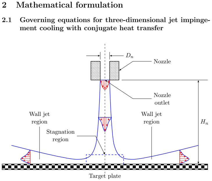
[Figure 1] The caption of Figure 1 describes a PINN architecture, but the figure appears to show the jet impingement geometry; the caption should be corrected, since the PINN architecture is displayed in Figure 3.
[Table 2 and Nomenclature] The Nomenclature defines α as thermal diffusivity, but Table 2 lists 'Thermal Conductivity αs: 16.27 W m−1 K−1'; the symbol for thermal conductivity should be κ_s, and the thermal diffusivity should be reported separately with consistent units.
[Section 2.2 and Section 3] There are typographical errors that should be corrected, including 'axis-symmetric' instead of 'axisymmetric' in Section 2.2 and 'follwoing' in the definition of the initial loss in Section 3.

Circularity Check

0 steps flagged · score 0.0 of 10

No circularity: the PINN estimates Bi_fc from sparse noisy solid temperatures, and the benchmark h_ref comes from an independent CHT simulation; the quadratic ansatz is a stated modeling assumption, not a definitional loop.

full rationale

The paper's derivation chain is self-contained and non-circular. The inverse problem in Section 2.2 estimates Bi_fc from sparse, noisy temperature data Tmeas generated by CHT simulations, while the benchmark href is the CHT-derived convective heat transfer profile used only in the error metric of Eq. (4.1). The PINN does not receive href as an input; Bi_fc is a trainable parameter learned from the temperature data, boundary, initial, and PDE losses. The constant-coefficient case compares the PINN estimate against a spatially averaged CHT value obtained by numerical integration, which is a genuine external benchmark rather than a refit of the PINN output. The spatially varying case assumes a second-degree polynomial for h_fc(x) in Section 5.2, and Table 4 indeed shows a zero-noise error floor around 6.1-6.4%; this reflects the approximation bias of the quadratic ansatz relative to the CHT profile and is a model limitation, not circularity, because the ansatz is stated explicitly and tested against an independent simulation. The paper also transparently acknowledges that CHT simulations are used as both benchmark and synthetic-data proxy, and that future work will address real experimental datasets. No load-bearing self-citations appear: the cited prior works for PINNs, DeepXDE, and the jet-impingement geometry are external references, and no uniqueness theorem is invoked to force the chosen functional form. Any concern about the adequacy of the quadratic profile for real impinging jets is a correctness or generalizability issue, not a circular-reasoning issue. Therefore the paper does not reduce any prediction to its inputs by construction.

Assumptions & free parameters 3 free parameters · 6 assumptions · 0 invented entities

The central claim depends on the fidelity of CHT-generated synthetic temperatures, the polynomial parameterization of the CHTC, and the assumed known free-convection coefficient; no new physical entities are introduced.

free parameters (3)

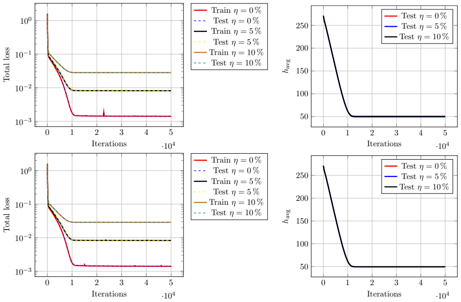
Bi_fc (constant CHTC) = not reported numerically; convergence plots show h_avg roughly 50-250 W/m2K
Trained as an external variable in the PINN loss; the inverse problem's target parameter.
Polynomial coefficients a0, a1, a2 for Bi_fc(x) = not reported
Define the spatially varying CHTC profile; fitted during PINN training in Section 5.2.
L2 regularization coefficient = not specified
Added to the loss 'that results in a smooth evolution' (Section 3); chosen by hand but its value is not given, affecting reproducibility.

assumptions (6)

domain assumption 2D transient heat conduction equation (Eq. 2.12-2.13) correctly describes the solid temperature field.
The inverse problem is built on this PDE; invoked in Sections 2.2 and 3.
domain assumption The convective boundary condition with h_fc(x) and h_fr (Eq. 2.14) is an accurate model of the fluid-solid interface; h_fr is presumed known.
The unknown CHTC enters only through this boundary condition; the known free convection coefficient is stated as presumed known in Section 2.2.
domain assumption Axisymmetry reduces the 3D disc to a 2D slice with a symmetry condition at x=0.
The paper assumes a perfectly symmetric jet and uses a thin central slice; stated in Section 2.2 and Figure 2.
domain assumption The CHT simulation with the RNG k-epsilon model provides a faithful ground truth for both temperatures and CHTC.
All validation is against synthetic CHT data; the paper acknowledges this is a surrogate for experiments in Section 2.1.
ad hoc to paper The second-degree polynomial ansatz for h_fc(x) spans the true spatial profile.
Section 5.2 assumes this functional form; no test with a non-quadratic profile is provided, so the central spatially varying claim depends on this restriction.
domain assumption Known, temperature-independent material properties for stainless steel (rho_s, cp_s, kappa_s).
Listed in Table 2 and used in the heat equation and boundary conditions.

how reviews work

0 comments

Cite this review

Pith. "Pith review of Physics-Informed Neural Networks for Estimating Convective Heat Transfer in Jet Impingement Cooling: A Comparison with Conjugate Heat Transfer Simulations." pith.science (2026). https://pith.science/paper/7XCH7UTG

@misc{pith2026250709356,
  author       = {Pith},
  title        = {Pith review of: Physics-Informed Neural Networks for Estimating Convective Heat Transfer in Jet Impingement Cooling: A Comparison with Conjugate Heat Transfer Simulations},
  year         = {2026},
  howpublished = {\url{https://pith.science/paper/7XCH7UTG}},
  note         = {Machine review of arXiv:2507.09356}
}

read the original abstract

Efficient cooling is vital for the performance and reliability of modern systems such as electronics, nuclear reactors, and industrial equipment. Jet impingement cooling is widely used for its high local heat transfer rates. Accurate estimation of convective heat transfer coefficient (CHTC) is essential for design, simulation, and control of thermal systems. However, estimating spatially varying CHTCs from limited and noisy temperature data poses a challenging inverse problem. This study presents a physics-informed neural network (PINN) framework to estimate both averaged and spatially varying CHTCs at the fluid-solid interface in a jet impingement setup at Reynolds number 5000. The model uses sparse and noisy temperature data from within the solid and embeds the transient heat conduction equation along with boundary and initial conditions into its loss function. This enables inference of unknown boundary parameters without explicit modeling of the fluid domain. Validation is performed using synthetic temperature data from high-fidelity conjugate heat transfer (CHT) simulations. The framework is tested under various additive Gaussian noise levels (up to 30 percent) and sampling rates 0.25 to 4.0 per second. For noise levels up to 10% and sampling rates of 0.5 per second or higher, estimated CHTCs match CHT-derived benchmarks with relative errors below 8 percent. Even under high-noise scenarios, the framework maintains predictive accuracy when time resolution is sufficient. These results highlight the method's robustness to noise and sparse data, offering a scalable alternative to traditional inverse methods, experimental measurements, or full CHT modeling for estimating boundary thermal parameters in real-world cooling applications.

Figures

Figures reproduced from arXiv: 2507.09356 by the authors.

**Figure 2.** Left panel: Schematic of the jet impingement cooling of a thin disc with radius R and thickness L. Right panel: Computational domain and boundary conditions used for inverse analysis. Owing to the axisymmetry of the centrally impinging jet, a representative 2D slice is extracted to enable estimation of the convective heat transfer coefficient over the entire domain. The magnified view on the right illustrates the a… view at source ↗

**Figure 3.** Architecture of a Physics-Informed Neural Network (PINN) for [PITH_FULL_IMAGE:figures/full_fig_p014_3.png] view at source ↗

Figures from the paper (8 more)

**Figure 4.** Figure 4: Schematic of the front view of the computational domain used for [PITH_FULL_IMAGE:figures/full_fig_p018_4.png]

**Figure 5.** Figure 5: Convergence plots of total loss for both training and test data [PITH_FULL_IMAGE:figures/full_fig_p023_5.png]

**Figure 6.** Figure 6: Convergence plots of total loss for both training and test data [PITH_FULL_IMAGE:figures/full_fig_p024_6.png]

**Figure 7.** Figure 7: Estimated profiles of the convective heat transfer coefficient [PITH_FULL_IMAGE:figures/full_fig_p029_7.png]

**Figure 8.** Figure 8: Estimated profiles of the convective heat transfer coefficient on [PITH_FULL_IMAGE:figures/full_fig_p030_8.png]

**Figure 9.** Figure 9: Convergence plots of total loss for both training and test data (left) [PITH_FULL_IMAGE:figures/full_fig_p031_9.png]

**Figure 10.** Figure 10: Convergence plots of total loss for both training and test data [PITH_FULL_IMAGE:figures/full_fig_p032_10.png]

**Figure 11.** Figure 11: Grid independence study showing the variation of spatial dis [PITH_FULL_IMAGE:figures/full_fig_p033_11.png]

Discussion (0). Continue with ORCID to comment.

Reference graph

Works this paper leans on

44 extracted references · 35 canonical work pages

[1]

Rough surfaces with enhanced heat transfer for electronics cool- ing by direct metal laser sintering

Luigi Ventola, Francesco Robotti, Masoud Dialameh, Flaviana Calig- nano, Diego Manfredi, Eliodoro Chiavazzo, and Pietro Asinari. Rough surfaces with enhanced heat transfer for electronics cool- ing by direct metal laser sintering. International Journal of Heat and Mass Transfer , 75:58–74, August 2014. ISSN 00179310. doi: 10.1016/j.ijheatmasstransfer.2014...

work page doi:10.1016/j.ijheatmasstransfer.2014.03.037 2014
[2]

Mahajan, Chia-pin Chiu, and G

R. Mahajan, Chia-pin Chiu, and G. Chrysler. Cooling a Microprocessor Chip. Proceedings of the IEEE , 94(8):1476–1486, August 2006. ISSN 0018-9219, 1558-2256. doi: 10.1109/JPROC.2006.879800. URL http: //ieeexplore.ieee.org/document/1705137/

work page arXiv 2006
[3]

High Performance Loop Heat Pipe With Flat Evaporator for Energy-Saving Cool- ing Systems of Supercomputers

Zhi Hu Xue, Wei Qu, and Ming Hui Xie. High Performance Loop Heat Pipe With Flat Evaporator for Energy-Saving Cool- ing Systems of Supercomputers. Journal of Heat Transfer , 142(3):031901, March 2020. ISSN 0022-1481, 1528-8943. doi: 10.1115/1.4045730. URL https://asmedigitalcollection.asme. 34 org/heattransfer/article/doi/10.1115/1.4045730/1072097/ High-Pe...

work page doi:10.1115/1.4045730 2020
[4]

Recent Studies in Turbine Blade Cooling

Je-Chin Han. Recent Studies in Turbine Blade Cooling. International Journal of Rotating Machinery , 10(6):443–457, January 2004. ISSN 1023-621X, 1542-3034. doi: 10.1155/S1023621X04000442. URL https: //onlinelibrary.wiley.com/doi/10.1155/S1023621X04000442

work page doi:10.1155/s1023621x04000442 2004
[5]

Silk, Eric L

Eric A. Silk, Eric L. Golliher, and R. Paneer Selvam. Spray cool- ing heat transfer: Technology overview and assessment of future chal- lenges for micro-gravity application. Energy Conversion and Manage- ment, 49(3):453–468, March 2008. ISSN 01968904. doi: 10.1016/ j.enconman.2007.07.046. URL https://linkinghub.elsevier.com/ retrieve/pii/S0196890407003664

work page 2008
[6]

A comprehensive review of advances in physics-informed neural networks and their applications in complex fluid dynamics

Chi Zhao, Feifei Zhang, Wenqiang Lou, Xi Wang, and Jianyong Yang. A comprehensive review of advances in physics-informed neural networks and their applications in complex fluid dynamics. Physics of Fluids , 36 (10):101301, October 2024. ISSN 1070-6631, 1089-7666. doi: 10.1063/5. 0226562. URL https://pubs.aip.org/pof/article/36/10/101301/ 3315125/A-compreh...

doi:10.1063/5 2024
[7]

Sengupta, B

J. Sengupta, B. G. Thomas, and M. A. Wells. The use of water cooling during the continuous casting of steel and aluminum alloys. Metal- lurgical and Materials Transactions A , 36(1):187–204, January 2005. ISSN 1073-5623, 1543-1940. doi: 10.1007/s11661-005-0151-y. URL https://link.springer.com/10.1007/s11661-005-0151-y

work page doi:10.1007/s11661-005-0151-y 2005
[8]

General principles of controlled water cooling for metallurgical on-line hot rolling processes: forced flow and sprayed surfaces with film boiling regime and rewetting phenomena

Jos´ e Rivallin and St´ ephane Viannay. General principles of controlled water cooling for metallurgical on-line hot rolling processes: forced flow and sprayed surfaces with film boiling regime and rewetting phenomena. International Journal of Thermal Sciences , 40(3):263–272, March 2001. ISSN 12900729. doi: 10.1016/S1290-0729(00)01216-3. URL https: //lin...

work page doi:10.1016/s1290-0729(00)01216-3 2001

Show all 44 references

[9]

Mazzaferro, Filippo Montevecchi, and Gianni Campatelli

William Hackenhaar, Jos´ e A.E. Mazzaferro, Filippo Montevecchi, and Gianni Campatelli. An experimental-numerical study of active cooling in wire arc additive manufacturing. Journal of Manufacturing Pro- cesses, 52:58–65, April 2020. ISSN 15266125. doi: 10.1016/j.jmapro. 2020....

2020 doi
[10]

Adaptive Control of Data Center Cooling using Deep Reinforcement Learning

Albin Heimerson, Johannes Sjolund, Rickard Brannvall, Jonas Gustafs- son, and Johan Eker. Adaptive Control of Data Center Cooling using Deep Reinforcement Learning. In 2022 IEEE International Confer- ence on Autonomic Computing and Self-Organizing Systems Compan- ion (ACSOS-C)...

2022
[11]

Zuckerman and N

N. Zuckerman and N. Lior. Jet Impingement Heat Transfer: Physics, Correlations, and Numerical Modeling. In Advances in Heat Trans- fer, volume 39, pages 565–631. Elsevier, 2006. ISBN 978-0-12-020039-

2006
[12]

URL https://linkinghub

doi: 10.1016/S0065-2717(06)39006-5. URL https://linkinghub. elsevier.com/retrieve/pii/S0065271706390065

doi
[13]

Infrared ther- mography for convective heat transfer measurements

Giovanni Maria Carlomagno and Gennaro Cardone. Infrared ther- mography for convective heat transfer measurements. Experiments in Fluids, 49(6):1187–1218, December 2010. ISSN 0723-4864, 1432-1114. doi: 10.1007/s00348-010-0912-2. URL http://link.springer.com/ 10.1007/s00348-010-0912-2

2010 doi
[14]

Bountin, Boris V

Helmut Knauss, Tim Roediger, Dimitry A. Bountin, Boris V. Smorod- sky, Anatoly A. Maslov, and Julio Srulijes. Novel Sensor for Fast Heat Flux Measurements. Journal of Spacecraft and Rockets, 46(2):255–265, March 2009. ISSN 0022-4650, 1533-6794. doi: 10.2514/1.32011. URL https:...

2009 doi
[15]

An in-depth analysis of conjugate heat transfer process of impingement jet

Xiao Wei Zhu, Lei Zhu, and Jing Quan Zhao. An in-depth analysis of conjugate heat transfer process of impingement jet. International Journal of Heat and Mass Transfer, 104:1259–1267, January 2017. ISSN 00179310. doi: 10.1016/j.ijheatmasstransfer.2016.09.075. URL https: //linki...

2017 doi
[16]

Numerical study of transient con- jugate heat transfer of a turbulent impinging jet

Yue-Tzu Yang and Shiang-Yi Tsai. Numerical study of transient con- jugate heat transfer of a turbulent impinging jet. International Jour- nal of Heat and Mass Transfer , 50(5-6):799–807, March 2007. ISSN 00179310. doi: 10.1016/j.ijheatmasstransfer.2006.08.022. URL https: //lin...

2007 doi
[17]

Necati ¨Ozi¸ sik and Helcio R

M. Necati ¨Ozi¸ sik and Helcio R. B. Orlande.Inverse heat transfer: fun- damentals and applications . Heat transfer series. CRC Press, Taylor & Francis Group, Boca Raton London New York, second edition edition,
[18]

Inverse analysis for transient thermal load identification and application to aerodynamic heating on atmospheric reentry capsule

Toshiya Nakamura, Yukihiro Kamimura, Hirotaka Igawa, and Yoshiki Morino. Inverse analysis for transient thermal load identification and application to aerodynamic heating on atmospheric reentry capsule. Aerospace Science and Technology , 38:48–55, October 2014. ISSN 12709638. ...

2014 doi
[20]

Mold transient heat transfer behavior based on measurement and inverse analysis of slab continuous casting

Xudong Wang, Ling Tang, Xinyang Zang, and Man Yao. Mold transient heat transfer behavior based on measurement and inverse analysis of slab continuous casting. Journal of Materials Process- ing Technology, 212(9):1811–1818, September 2012. ISSN 09240136. doi: 10.1016/j.jmatprot...

2012 doi
[21]

Luchesi and Reginaldo T

Vanda M. Luchesi and Reginaldo T. Coelho. An inverse method to estimate the moving heat source in machining process. Applied Ther- mal Engineering , 45-46:64–78, December 2012. ISSN 13594311. doi: 10.1016/j.applthermaleng.2012.04.014. URL https://linkinghub. elsevier.com/retri...

2012 doi
[22]

Viloche Baz´ an, and Leonardo S

Fabio Bozzoli, Luca Cattani, Sara Rainieri, Ferm ´ ın S. Viloche Baz´ an, and Leonardo S. Borges. Estimation of the local heat-transfer coefficient in the laminar flow regime in coiled tubes by the Tikhonov regularisa- tion method. International Journal of Heat and Mass Transf...

2014 doi
[23]

3D- transient identification of surface heat sources through infrared ther- mography measurements on the rear face

Jean-Gabriel Bauzin, S´ ebastien Vintrou, and Najib Laraqi. 3D- transient identification of surface heat sources through infrared ther- mography measurements on the rear face. International Journal of Thermal Sciences , 148:106115, February 2020. ISSN 12900729. doi: 10.1016/j....

2020
[24]

Inverse solutions to a vertical plate cooling in air – a comparative study

Zbigniew Malinowski, Beata Hada la, and Agnieszka Cebo-Rudnicka. Inverse solutions to a vertical plate cooling in air – a comparative study. International Journal of Heat and Mass Transfer , 188:122636, June 2022. ISSN 00179310. doi: 10.1016/j.ijheatmasstransfer.2022. 122636. ...

2022 doi
[25]

Han, H.B

W.W. Han, H.B. Chen, and T. Lu. Estimation of the time-dependent convective boundary condition in a horizontal pipe with thermal strat- ification based on inverse heat conduction problem. International Journal of Heat and Mass Transfer , 132:723–730, April 2019. ISSN 00179310....

2019 doi
[26]

Evans, Hywel Thomas, and Perumal Nithiarasu

Hamid Reza Tamaddon-Jahromi, Neeraj Kavan Chakshu, Igor Sazonov, Llion M. Evans, Hywel Thomas, and Perumal Nithiarasu. Data-driven inverse modelling through neural network (deep learning) and compu- tational heat transfer. Computer Methods in Applied Mechanics and Engineering,...

2020
[27]

Curtis R. Vogel. Computational methods for inverse problems. Frontiers in applied mathematics. Society for Industrial and Applied Mathemat- ics, Philadelphia, 2002. ISBN 978-0-89871-507-1

2002
[28]

Lagaris, A

I.E. Lagaris, A. Likas, and D.I. Fotiadis. Artificial neural networks for solving ordinary and partial differential equations. IEEE Trans- actions on Neural Networks , 9(5):987–1000, September 1998. ISSN 10459227. doi: 10.1109/72.712178. URL http://ieeexplore.ieee. org/documen...

1998 doi
[29]

Woodbury, and Gyula Gr´ of

Bal´ azs Cz´ el, Keith A. Woodbury, and Gyula Gr´ of. Simultaneous es- timation of temperature-dependent volumetric heat capacity and ther- mal conductivity functions via neural networks. International Journal of Heat and Mass Transfer, 68:1–13, January 2014. ISSN 00179310. do...

2014 doi
[30]

Scientific Machine Learning Through Physics–Informed Neural Networks: Where we are and What’s Next

Salvatore Cuomo, Vincenzo Schiano Di Cola, Fabio Giampaolo, Gian- luigi Rozza, Maziar Raissi, and Francesco Piccialli. Scientific Machine Learning Through Physics–Informed Neural Networks: Where we are and What’s Next. Journal of Scientific Computing, 92(3):88, September
[31]

Raissi, P

M. Raissi, P. Perdikaris, and G.E. Karniadakis. Physics-informed neural networks: A deep learning framework for solving forward and inverse problems involving nonlinear partial differential equations. Journal of 38 Computational Physics , 378:686–707, February 2019. ISSN 00219...

2019 doi
[32]

Witschey, John A

Georgios Kissas, Yibo Yang, Eileen Hwuang, Walter R. Witschey, John A. Detre, and Paris Perdikaris. Machine learning in cardiovascu- lar flows modeling: Predicting arterial blood pressure from non-invasive 4D flow MRI data using physics-informed neural networks. Computer Metho...
[33]

A physics- informed deep learning method for solving direct and inverse heat con- duction problems of materials

Zhili He, Futao Ni, Weiguo Wang, and Jian Zhang. A physics- informed deep learning method for solving direct and inverse heat con- duction problems of materials. Materials Today Communications , 28: 102719, September 2021. ISSN 23524928. doi: 10.1016/j.mtcomm. 2021.102719. URL...

2021
[34]

S. B. Pope. Turbulent flows. Cambridge University Press, Cambridge ; New York, 2000. ISBN 978-0-521-59125-6 978-0-521-59886-6

2000
[35]

Deep- XDE: A Deep Learning Library for Solving Differential Equations

Lu Lu, Xuhui Meng, Zhiping Mao, and George Em Karniadakis. Deep- XDE: A Deep Learning Library for Solving Differential Equations. SIAM Review , 63(1):208–228, January 2021. ISSN 0036-1445, 1095-

2021
[36]

TensorFlow: a system for Large-Scale ma- chine learning

Mart ´ ın Abadi, Paul Barham, Jianmin Chen, Zhifeng Chen, Andy Davis, Jeffrey Dean, Matthieu Devin, Sanjay Ghemawat, Geoffrey Irving, Michael Isard, and others. TensorFlow: a system for Large-Scale ma- chine learning. In 12th USENIX symposium on operating systems design and im...

2016
[37]

Practical bayesian optimization of machine learning algorithms

Jasper Snoek, Hugo Larochelle, and Ryan P Adams. Practical bayesian optimization of machine learning algorithms. Advances in neural infor- mation processing systems, 25, 2012

2012
[38]

Experimental and numeri- cal study on the transient heat-transfer characteristics of circular air- jet impingement on a flat plate

Qiang Guo, Zhi Wen, and Ruifeng Dou. Experimental and numeri- cal study on the transient heat-transfer characteristics of circular air- jet impingement on a flat plate. International Journal of Heat and Mass Transfer , 104:1177–1188, January 2017. ISSN 00179310. doi: 10.1016/j...

2017 doi
[39]

Fern´ andez-Mart ´ ınez, J.L.G

J.L. Fern´ andez-Mart ´ ınez, J.L.G. Pallero, Z. Fern´ andez-Mu˜ niz, and L.M. Pedruelo-Gonz´ alez. The effect of noise and Tikhonov’s regulariza- tion in inverse problems. Part I: The linear case. Journal of Ap- plied Geophysics, 108:176–185, September 2014. ISSN 0926-9851. d...

2014 doi
[40]

Engl, Martin Hanke, and Andreas Neubauer

Heinz W. Engl, Martin Hanke, and Andreas Neubauer. Regularization of inverse problems. Number v. 375 in Mathematics and its applications. Kluwer Academic Publishers, Dordrecht ; Boston, 1996. ISBN 978-0- 7923-4157-4. 40

1996
[43]

Optuna: A next-generation hyperparameter opti- mization framework

Takuya Akiba, Shotaro Sano, Toshihiko Yanase, Takeru Ohta, and Masanori Koyama. Optuna: A next-generation hyperparameter opti- mization framework. In The 25th ACM SIGKDD International Confer- ence on Knowledge Discovery & Data Mining , pages 2623–2631, 2019

2019
[2020]

doi: 10.1016/j.cma.2019.112623

ISSN 00457825. doi: 10.1016/j.cma.2019.112623. URL https: //linkinghub.elsevier.com/retrieve/pii/S0045782519305055

2019
[2021]

ISBN 978-1-00-315515-7 978-0-367-82067-1 978-0-367-72526-6. 36
[2022]

doi: 10.1007/s10915-022-01939-z

ISSN 0885-7474, 1573-7691. doi: 10.1007/s10915-022-01939-z. URL https://link.springer.com/10.1007/s10915-022-01939-z

doi
[7200]

URL https://epubs.siam.org/doi/ 10.1137/19M1274067

doi: 10.1137/19M1274067. URL https://epubs.siam.org/doi/ 10.1137/19M1274067. 39

doi

Pith tools

Reviewed August 6, 2026 · model on record in the stance chip above.

[1] [1]

Rough surfaces with enhanced heat transfer for electronics cool- ing by direct metal laser sintering

Luigi Ventola, Francesco Robotti, Masoud Dialameh, Flaviana Calig- nano, Diego Manfredi, Eliodoro Chiavazzo, and Pietro Asinari. Rough surfaces with enhanced heat transfer for electronics cool- ing by direct metal laser sintering. International Journal of Heat and Mass Transfer , 75:58–74, August 2014. ISSN 00179310. doi: 10.1016/j.ijheatmasstransfer.2014...

work page doi:10.1016/j.ijheatmasstransfer.2014.03.037 2014

[2] [2]

Mahajan, Chia-pin Chiu, and G

R. Mahajan, Chia-pin Chiu, and G. Chrysler. Cooling a Microprocessor Chip. Proceedings of the IEEE , 94(8):1476–1486, August 2006. ISSN 0018-9219, 1558-2256. doi: 10.1109/JPROC.2006.879800. URL http: //ieeexplore.ieee.org/document/1705137/

work page arXiv 2006

[3] [3]

High Performance Loop Heat Pipe With Flat Evaporator for Energy-Saving Cool- ing Systems of Supercomputers

Zhi Hu Xue, Wei Qu, and Ming Hui Xie. High Performance Loop Heat Pipe With Flat Evaporator for Energy-Saving Cool- ing Systems of Supercomputers. Journal of Heat Transfer , 142(3):031901, March 2020. ISSN 0022-1481, 1528-8943. doi: 10.1115/1.4045730. URL https://asmedigitalcollection.asme. 34 org/heattransfer/article/doi/10.1115/1.4045730/1072097/ High-Pe...

work page doi:10.1115/1.4045730 2020

[4] [4]

Recent Studies in Turbine Blade Cooling

Je-Chin Han. Recent Studies in Turbine Blade Cooling. International Journal of Rotating Machinery , 10(6):443–457, January 2004. ISSN 1023-621X, 1542-3034. doi: 10.1155/S1023621X04000442. URL https: //onlinelibrary.wiley.com/doi/10.1155/S1023621X04000442

work page doi:10.1155/s1023621x04000442 2004

[5] [5]

Silk, Eric L

Eric A. Silk, Eric L. Golliher, and R. Paneer Selvam. Spray cool- ing heat transfer: Technology overview and assessment of future chal- lenges for micro-gravity application. Energy Conversion and Manage- ment, 49(3):453–468, March 2008. ISSN 01968904. doi: 10.1016/ j.enconman.2007.07.046. URL https://linkinghub.elsevier.com/ retrieve/pii/S0196890407003664

work page 2008

[6] [6]

A comprehensive review of advances in physics-informed neural networks and their applications in complex fluid dynamics

Chi Zhao, Feifei Zhang, Wenqiang Lou, Xi Wang, and Jianyong Yang. A comprehensive review of advances in physics-informed neural networks and their applications in complex fluid dynamics. Physics of Fluids , 36 (10):101301, October 2024. ISSN 1070-6631, 1089-7666. doi: 10.1063/5. 0226562. URL https://pubs.aip.org/pof/article/36/10/101301/ 3315125/A-compreh...

doi:10.1063/5 2024

[7] [7]

Sengupta, B

J. Sengupta, B. G. Thomas, and M. A. Wells. The use of water cooling during the continuous casting of steel and aluminum alloys. Metal- lurgical and Materials Transactions A , 36(1):187–204, January 2005. ISSN 1073-5623, 1543-1940. doi: 10.1007/s11661-005-0151-y. URL https://link.springer.com/10.1007/s11661-005-0151-y

work page doi:10.1007/s11661-005-0151-y 2005

[8] [8]

General principles of controlled water cooling for metallurgical on-line hot rolling processes: forced flow and sprayed surfaces with film boiling regime and rewetting phenomena

Jos´ e Rivallin and St´ ephane Viannay. General principles of controlled water cooling for metallurgical on-line hot rolling processes: forced flow and sprayed surfaces with film boiling regime and rewetting phenomena. International Journal of Thermal Sciences , 40(3):263–272, March 2001. ISSN 12900729. doi: 10.1016/S1290-0729(00)01216-3. URL https: //lin...

work page doi:10.1016/s1290-0729(00)01216-3 2001