REVIEW 4 major objections 6 minor 91 references
Multi-Head Neural Operator for Modelling Interfacial Dynamics
T0 review · 4 major / 6 minor · reviewed 2026-08-06 · deepseek-v4-flash
Pith's one-line read The paper claims that a neural operator with time-specific output heads and step-to-step coupling can predict the full time evolution of phase-field PDEs in one forward pass, with lower error and cost than FNO-2d and FNO-3d.
desk verdict The MHNO architecture idea is genuinely useful, but the headline comparison is compromised by an unspecified and likely broken FNO-2d protocol under Approach III. read the letter →
The pith
A machine-rendered reading of the paper's core claim, the machinery that carries it, and where it could break.
The reading
What carries the argument
The load-bearing object is the pair $\{Q_n\}_{n=1}^{N_t}$ and $\{H_n\}_{n=2}^{N_t}$: time-specific projection operators replace the fixed output projection $Q$, and temporal coupling operators implement a message-passing-style recurrence between adjacent outputs. The shared Fourier backend (lift $P$, kernel layers $W_\ell + K_\ell$, activation) is evaluated once; each $Q_n$ maps the terminal latent representation to the field at time $t_n$, and each $H_n$ adds a learned contribution from the previous predicted field, so information flows forward in a way that mirrors causality. This design is what lets a single forward pass cover the full horizon while keeping parameter growth roughly linear rather than multiplicative in $N_t$.
What would settle it
Re-run the Cahn-Hilliard Approach III experiment with FNO-2d under an expanded hyperparameter search or longer training and check whether its test L2 error stays near 90%; if a reasonably tuned FNO-2d closes most of the gap to MHNO's roughly 2.5% error, the superiority claim is not sustained.
Extended reading notes
Core claim
On the paper's own terms, the discovery is that temporal structure in neural operators is best handled at the output, not by unrolling in time or by inflating the input into space-time. MHNO writes the solution map as $G_\theta(x,t_n)(a) = Q_n \circ (W_L + K_L) \circ \cdots \circ \sigma(W_1 + K_1) \circ P(a) + H_n \circ G_\theta(x,t_{n-1})(a)$, where each $Q_n$ is a projection neural network specialized to time step $n$ and each $H_n$ carries the previous predicted field into the current step. Because the shared Fourier layers are evaluated once and the heads are cheap, one forward pass yields all $N_t$ snapshots; because $H_n$ couples adjacent steps, the model has an explicit temporal prior without a 3D tensor. The paper further shows that setting all $H_n$ to zero recovers a standard neural operator, so MHNO inherits the universal-approximation guarantee for neural operators, and derives a bound $\|G_\theta(a;t_n)\|_U \le 4M$ when the output heads have norm at most 1 and the coupling maps have norm below 1. Empirically, on five phase-field benchmarks, MHNO reports the lowest test L2 errors across the three training approaches in most configurations, with particularly large gaps in the full-trajectory regime where FNO-2d sometimes exceeds 70-90% error.
Load-bearing premise
The comparison assumes FNO-2d and FNO-3d were tuned and trained as diligently as MHNO, so the huge baseline errors (about 90% on Cahn-Hilliard, 77% on MBE under Approach III) reflect the methods rather than their training setup; it also assumes the spectral reference solutions are accurate enough to serve as ground truth.
Editorial extensions
If this is right
- Inference cost for a full trajectory is nearly independent of horizon: one pass over the shared backbone plus cheap per-step heads, instead of $N_t$ sequential network evaluations or one $N_t$-times-larger convolution.
- Training on full trajectories (Approach III) becomes usable and is reported as the best regime for Allen-Cahn, Cahn-Hilliard, phase-field crystal, and molecular beam epitaxy, whereas FNO-2d degrades sharply in that regime.
- Parameter count grows only modestly with the number of time steps, since no time dimension is replicated through the whole network.
- Because standard neural operators are a special case (all $H_n=0$ and $Q_n=Q$), any approximation guarantee for standard neural operators applies to MHNO.
- The same architecture extends beyond 2D: the paper demonstrates it on 3D Allen-Cahn where the FNO baselines become computationally prohibitive.
Reading between the lines
- A natural stress test would swap MHNO's message-passing step for a single shared $Q$ head with $N_t$ output channels; if accuracy stays similar, the temporal coupling, not the multiple heads, may not be the source of gains.
- The architecture is generic enough that it should transfer to other stiff time-dependent PDEs, such as reaction-diffusion systems or turbulent flows, but the paper only demonstrates phase-field benchmarks, so that transfer is unverified.
- The reported failures of FNO-2d under Approach III are so large (roughly 90% L2 error on Cahn-Hilliard) that they raise the question of whether the baselines were given a comparable tuning budget; a controlled re-run would clarify whether the gap is architectural or operational.
- One could hybridize MHNO with a physics-informed loss by adding residual PDE terms in the $H_n$ connections, but the paper does not explore this; the architecture's explicit step coupling makes such a test natural.
Editorial analysis
A structured set of objections, weighed in public.
Referee Report
Summary. The paper proposes the Multi-Head Neural Operator (MHNO), a modification of the Fourier Neural Operator for time-dependent PDEs. Instead of a single global projection operator Q after the final latent representation, MHNO uses time-step-specific projection networks Q_n and explicit temporal coupling networks H_n between consecutive output heads, so that the model outputs all N_t snapshots in one forward pass while retaining sequential dependence. The authors claim an approximation theorem and a stability bound for the architecture, and they benchmark MHNO against FNO-2d and FNO-3d on five phase-field problems: Allen-Cahn, Cahn-Hilliard, Swift-Hohenberg, phase-field crystal, and molecular beam epitaxy, under three temporal training strategies (windowed, two-window, and full-trajectory). The reported results show MHNO generally achieving lower L2 test errors, fewer parameters, and shorter training times than the two baselines.
Significance. If the claims are correct, MHNO is a practically useful contribution: it offers a simple way to extend operator learning to long temporal horizons without the error accumulation of iterated one-step models or the parameter inflation of space-time FNO-3d. The paper has several concrete strengths: it uses an independent Fourier spectral solver to generate ground-truth data, so the benchmarking is not circular; it covers five distinct phase-field equations with different mathematical structure; it compares three training protocols; and it makes code and data publicly available. However, the theoretical support for MHNO is currently incomplete, and the most striking empirical advantage—especially under Approach III—rests on baseline results that are not adequately explained. The central architectural idea is plausible and the evidence base is broad, but the paper needs substantial clarification and correction before the superiority claim can be accepted.
major comments (4)
- [Section 3, Eq. (7)] The bound in Eq. (7) is asserted without a proof. The assumptions ||Q_n|| <= 1 and ||H_n|| <= gamma < 1 control only the projection and coupling operators; they do not control the norm of the latent representation v_T, which enters the recurrence G_n = Q_n v_T + H_n G_{n-1}. Without a bound on ||v_T||, or an argument that the approximation error in Eq. (6) can be used to control it, the claimed uniform bound ||G_theta(a;t_n)||_U <= 4M does not follow. The authors should either provide a complete proof or state a corrected theorem with the additional hypothesis needed.
- [Section 3, Theorem 1 and Eq. (5)] The containment argument that derives the approximation theorem is not established as written. Setting H_n = O and all Q_n = Q makes the MHNO output N_t identical copies of the same field, which cannot approximate a nontrivial trajectory in the product space U^{N_t}. To inherit the universal approximation theorem from standard neural operators, the authors must specify the target space and norm for the joint map a -> (u_1,...,u_{N_t}) and prove componentwise approximation (for example, by applying [70, Thm. 11] to each time-specific component with its own Q_n). As it stands, the theorem overstates what the containment argument shows.
- [Section 4, Approach III; Tables 2 and 5; Appendix B] The protocol for FNO-2d under Approach III is unspecified. Approach III is defined as the direct mapping phi_0 -> (phi_1,...,phi_Nt), but Section 2 defines FNO-2d as a one-step-ahead iterator. The paper never states whether FNO-2d was given N_t output heads, unrolled with teacher forcing, or modified in some other way. The train L2 errors of 90.30 +/- 1.11% for Cahn-Hilliard (Table 2) and 76.12 +/- 10.70% for MBE (Table 5) are signatures of a model that failed to train, and no implementation detail rules out an ill-posed output head or a train/inference mismatch. The authors must specify the exact FNO-2d architecture, loss, teacher-forcing scheme, and inference procedure used for Approach III, or remove these rows from the comparison. Appendix B does not resolve the issue: Table 6 is captioned 'Approach I' while the surrounding text says the table covers Approach III, so the hyperparameter documentation for the crucial setting is internally inconsistent.
- [Tables 1-5] The reported parameter counts for FNO-3d are inconsistent with the stated architecture. FNO-3d's final output channel dimension must equal the number of predicted time slices, which differs across approaches (n_w = 10 for Approach I, N_t/2 for Approach II, and N_t = 90 or 100 for Approach III), yet the parameter count is identical across all three approaches for each equation (e.g., 4,197,937 in all rows of Table 1). This is not plausible unless the implementation shares output weights across approaches in a way that is not described. Please report the actual parameter counts or clarify how the three approaches are realized in FNO-3d, since the parameter-efficiency claim depends on these numbers.
minor comments (6)
- [Section 3, Eq. (8)] The notation |H_n| and |Q_n| in the definition of R_H^{(n)} is undefined; please specify whether these are operator norms, Frobenius norms, or absolute values of the network parameters, and justify the use of the exponential softmax-style weighting.
- [Table 2, Approach II row] The FNO-2d entry '8,00±5,47' uses a decimal comma while all other entries in the paper use decimal points; please unify the formatting.
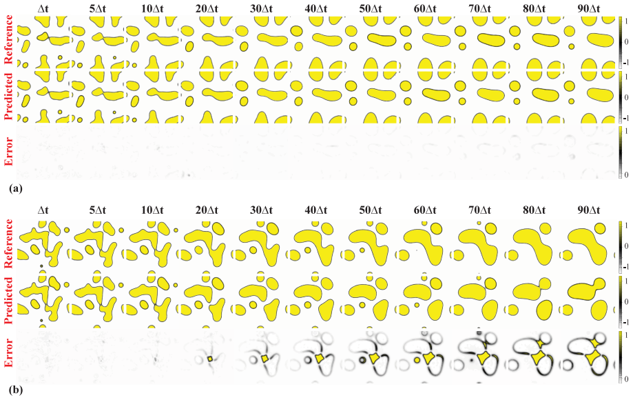
- [Figures 3, 4, 6, 7, 9, 11, 13] Several figure captions and colorbar labels are garbled, including strings like '1-101-10101-101-1010' and the repeated 'Reference Predicted' text in Figure 8; these need to be regenerated or cleaned before publication.
- [Section 2-3, notation] The notation in Eq. (4), 'G_theta(x,t_n)(a(x))', mixes the input function and the spatial variable awkwardly; write G_theta(a)(x,t_n) or an equivalent consistently throughout.
- [Introduction, Section 1] The statement that FNO-3d has 'no explicit connection between the solution fields at successive time steps' is inaccurate: the 3D convolution kernels in FNO-3d mix neighboring time slices in the hidden layers before the output projection. Please rephrase this motivation to avoid mischaracterizing the baseline.
- [Throughout] Minor typos include 'anthiphase' in Table 1's caption, 'Distibution' in Figure 5, 'T emp. Appr.' in the table headers, and 'we explored' in the Introduction; these should be corrected in a final pass.
Circularity Check
No substantive circularity: MHNO's empirical claims rest on external spectral-reference benchmarks, and the approximation theorem is imported from external prior work, so no load-bearing step reduces to its own input.
full rationale
The central claim is that replacing the global projection Q in Eq. (3) with time-specific projections {Q_n} and temporal couplings {H_n} in Eq. (4) lets a single neural operator output the full trajectory in one forward pass. This is an architectural proposal whose validation is external: the reference data are generated by a Fourier-spectral solver (Section 4, Appendix A), and the accuracy comparisons in Tables 1-5 are made against FNO-2d and FNO-3d on those independently generated trajectories. No fitted parameter is renamed as a prediction; the R_H metric of Eq. (8) is a post-hoc diagnostic of trained weights, not a forecast. The approximation theorem is explicitly inherited from Kovachki et al. [70], which is outside the author group, and it is not used as a self-citation chain to forbid alternatives. The paper's self-citations (e.g., [8], [11], [14], [40]-[42], [62]) appear in the literature background and are not load-bearing for the MHNO design or the numerical results. The weaknesses that do exist are non-circular: Appendix B says Table 6 concerns Approach III while the table caption says Approach I, and the paper never specifies how FNO-2d was configured under Approach III, whose reported near-90% train errors are likely a benchmarking or setup artifact. Similarly, the containment argument for Theorem 1 is logically questionable because a restricted subclass with all Q_n equal would emit identical time slices, but it relies on an external theorem and does not make the empirical claim equivalent to its inputs. Overall, the derivation chain is self-contained against independent benchmarks and does not exhibit circularity.
Assumptions & free parameters
free parameters (2)
- Per-model and per-approach hyperparameters (learning rate, widths M, W, W_Q, W_H, Fourier layers, modes, batch size… =
Examples: Allen-Cahn MHNO best config uses lr=0.001, M=12, W_Q=32, W_H=8, N_l=4, N_Q=2; full grid in Table 7
- Number of predicted output heads N_t or window length n_w =
10 (Approach I), 45 (Approach II), 90 or 100 (Approach III)
assumptions (4)
- standard math Universal approximation of standard neural operators (Kovachki et al., Theorem 11 and Assumptions 9-10)
- domain assumption Spectral reference solutions are accurate enough to serve as ground truth
- domain assumption Gaussian random field initial conditions cover the target application regime
- ad hoc to paper Norm bounds ||Q_n|| less than or equal to 1 and ||H_n|| less than gamma with gamma less than 1 in Theorem 1
Cite this review
Pith. "Pith review of Multi-Head Neural Operator for Modelling Interfacial Dynamics." pith.science (2026). https://pith.science/paper/WGYDN35C
@misc{pith2026250717763,
  author       = {Pith},
  title        = {Pith review of: Multi-Head Neural Operator for Modelling Interfacial Dynamics},
  year         = {2026},
  howpublished = {\url{https://pith.science/paper/WGYDN35C}},
  note         = {Machine review of arXiv:2507.17763}
}
read the original abstract
Interfacial dynamics underlie a wide range of phenomena, including phase transitions, microstructure coarsening, pattern formation, and thin-film growth, and are typically described by stiff, time-dependent nonlinear partial differential equations (PDEs). Traditional numerical methods, including finite difference, finite element, and spectral techniques, often become computationally prohibitive when dealing with high-dimensional problems or systems with multiple scales. Neural operators (NOs), a class of deep learning models, have emerged as a promising alternative by learning mappings between function spaces and efficiently approximating solution operators. In this work, we introduce the Multi-Head Neural Operator (MHNO), an extended neural operator framework specifically designed to address the temporal challenges associated with solving time-dependent PDEs. Unlike existing neural operators, which either struggle with error accumulation or require substantial computational resources for high-dimensional tensor representations, MHNO employs a novel architecture with time-step-specific projection operators and explicit temporal connections inspired by message-passing mechanisms. This design allows MHNO to predict all time steps after a single forward pass, while effectively capturing long-term dependencies and avoiding parameter overgrowth. We apply MHNO to solve various phase field equations, including antiphase boundary motion, spinodal decomposition, pattern formation, atomic scale modeling, and molecular beam epitaxy growth model, and compare its performance with existing NO-based methods. Our results show that MHNO achieves superior accuracy, scalability, and efficiency, demonstrating its potential as a next-generation computational tool for phase field modeling. The code and data supporting this work is publicly available at https://github.com/eshaghi-ms/MHNO.
Figures


Figures from the paper (11 more)




Reference graph
Works this paper leans on
-
[1]
L. Hashemi, M. Blunt, and H. Hajibeygi. “Pore-scale modelling and sensitivity analyses of hydrogen- brine multiphase flow in geological porous media”. In:Scientific reports11.1 (2021), p. 8348.doi: 10.1038/s41598-021-87490-7
-
[2]
An introduction to phase-field modeling of microstructure evolution
N. Moelans, B. Blanpain, and P. Wollants. “An introduction to phase-field modeling of microstructure evolution”. In:Calphad32.2 (2008), pp. 268–294.doi:10.1016/j.calphad.2007.11.003
-
[3]
Phase-field models in materials science
I. Steinbach. “Phase-field models in materials science”. In:Modelling and simulation in materials science and engineering17.7 (2009), p. 073001.doi:10.1088/0965-0393/17/7/073001
-
[4]
Interfacial dynamics with soluble surfactants: A phase-field two-phase flow model with variable densities
G. Zhu and A. Li. “Interfacial dynamics with soluble surfactants: A phase-field two-phase flow model with variable densities”. In:Advances in Geo-Energy Research4.1 (2020), pp. 86–98.doi:10.26804/ ager.2020.01.08. 31
2020
-
[5]
Quantitative phase-field modeling of solute trapping in rapid solidifi- cation
S. Kavousi and M. A. Zaeem. “Quantitative phase-field modeling of solute trapping in rapid solidifi- cation”. In:Acta Materialia205 (2021), p. 116562.doi:10.1016/j.actamat.2020.116562
arXiv 2021
-
[6]
Phase field modeling and computer implementation: A review
X. Zhuang et al. “Phase field modeling and computer implementation: A review”. In:Engineering Fracture Mechanics262 (2022), p. 108234.doi:10.1016/j.engfracmech.2021.107881
arXiv 2022
-
[7]
Phase field simulation of liquid phase separation with fluid flow
G. Tegze, T. Pusztai, and L. Gr´ an´ asy. “Phase field simulation of liquid phase separation with fluid flow”. In:Materials Science and Engineering: A413 (2005), pp. 418–422.doi:10.1016/j.msea.2005. 09.045
-
[8]
Isogeometric analysis of hydrodynamics of vesicles using a mono- lithic phase-field approach
N. Valizadeh and T. Rabczuk. “Isogeometric analysis of hydrodynamics of vesicles using a mono- lithic phase-field approach”. In:Computer Methods in Applied Mechanics and Engineering388 (2022), p. 114191.doi:10.1016/j.cma.2021.114191
Show all 91 references
-
[9]
Phase-field Navier–Stokes model for vesicle doublets hydro- dynamics in incompressible fluid flow
M. Ashour, N. Valizadeh, and T. Rabczuk. “Phase-field Navier–Stokes model for vesicle doublets hydro- dynamics in incompressible fluid flow”. In:Computer Methods in Applied Mechanics and Engineering 412 (2023), p. 116063.doi:10.1016/j.cma.2023.116063
2023
-
[10]
Hydrodynamics of multicomponent vesicles: A phase-field approach
Z. Wen et al. “Hydrodynamics of multicomponent vesicles: A phase-field approach”. In:Computer Methods in Applied Mechanics and Engineering432 (2024), p. 117390.doi:10.1016/j.cma.2024. 117390
2024 doi
-
[11]
A monolithic finite element method for phase-field mod- eling of fully Eulerian fluid–structure interaction
N. Valizadeh, X. Zhuang, and T. Rabczuk. “A monolithic finite element method for phase-field mod- eling of fully Eulerian fluid–structure interaction”. In:Computer Methods in Applied Mechanics and Engineering435 (2025), p. 117618.doi:10.1016/j.cma.2024.117618
2025
-
[12]
Phase-field models for microstructure evolution
L.-Q. Chen. “Phase-field models for microstructure evolution”. In:Annual review of materials research 32.1 (2002), pp. 113–140.doi:10.1146/annurev.matsci.32.112001.132041
2002
-
[13]
Interface-tracking and interface-capturing techniques for finite element computation of moving boundaries and interfaces
T. E. Tezduyar. “Interface-tracking and interface-capturing techniques for finite element computation of moving boundaries and interfaces”. In:Computer Methods in Applied Mechanics and Engineering 195.23-24 (2006), pp. 2983–3000.doi:10.1016/j.cma.2004.09.018
2006 doi
-
[14]
Isogeometric analysis for phase-field models of geometric PDEs and high-order PDEs on stationary and evolving surfaces
N. Valizadeh and T. Rabczuk. “Isogeometric analysis for phase-field models of geometric PDEs and high-order PDEs on stationary and evolving surfaces”. In:Computer Methods in Applied Mechanics and Engineering351 (2019), pp. 599–642.doi:10.1016/j.cma.2019.03.043
2019 doi
-
[15]
Accelerating phase-field-based mi- crostructure evolution predictions via surrogate models trained by machine learning methods
D. Montes de Oca Zapiain, J. A. Stewart, and R. Dingreville. “Accelerating phase-field-based mi- crostructure evolution predictions via surrogate models trained by machine learning methods”. In:npj Computational Materials7.1 (2021), p. 3.doi:10.1038/s41524-020-00471-8
2021 doi
-
[16]
A spectral element-based phase field method for incompressible two-phase flows
Y. Xiao et al. “A spectral element-based phase field method for incompressible two-phase flows”. In: Physics of Fluids34.2 (2022).doi:10.1063/5.0077372. 32
2022 doi
-
[17]
A comparative review of XFEM, mixed FEM and phase-field models for quasi- brittle cracking
M. Cervera et al. “A comparative review of XFEM, mixed FEM and phase-field models for quasi- brittle cracking”. In:Archives of Computational Methods in Engineering29.2 (2022), pp. 1009–1083. doi:10.1007/s11831-021-09604-8
2022 doi
-
[18]
Learning two-phase microstructure evolution using neural operators and autoen- coder architectures
V. Oommen et al. “Learning two-phase microstructure evolution using neural operators and autoen- coder architectures”. In:npj Computational Materials8.1 (2022), p. 190.doi:10.1038/s41524-022- 00876-7
2022 doi
-
[19]
R. C. Smith.Uncertainty quantification: theory, implementation, and applications. SIAM, 2024.doi: 10.1137/1.9781611973228
2024 doi
-
[20]
Non-linear model reduction for uncertainty quantification in large-scale inverse problems
D. Galbally et al. “Non-linear model reduction for uncertainty quantification in large-scale inverse problems”. In:International journal for numerical methods in engineering81.12 (2010), pp. 1581– 1608.doi:10.1002/nme.2746
2010 doi
-
[21]
A dual mesh method with adaptivity for stress-constrained topology optimization
D. A. White, Y. Choi, and J. Kudo. “A dual mesh method with adaptivity for stress-constrained topology optimization”. In:Structural and Multidisciplinary Optimization61.2 (2020), pp. 749–762. doi:10.1007/s00158-019-02393-6
2020 doi
-
[22]
Accelerating Phase Field Simulations Through a Hybrid Adaptive Fourier Neural Operator with U-Net Backbone
C. Bonneville et al. “Accelerating Phase Field Simulations Through a Hybrid Adaptive Fourier Neural Operator with U-Net Backbone”. In:arXiv preprint arXiv:2406.17119(2024).doi:arXiv : 2406 . 17119v2
2024 arXiv
-
[23]
An efficient algorithm for 3D adaptive meshing
P. George, H. Borouchaki, and P. Laug. “An efficient algorithm for 3D adaptive meshing”. In:Advances in Engineering Software33.7-10 (2002), pp. 377–387.doi:10.1016/S0965-9978(02)00065-0
2002 doi
-
[24]
Machine-learning-based data-driven discovery of nonlinear phase-field dynamics
E. Kiyani et al. “Machine-learning-based data-driven discovery of nonlinear phase-field dynamics”. In: Physical Review E106.6 (2022), p. 065303.doi:10.1103/PhysRevE.106.065303
2022 doi
-
[25]
Bayesian deep convolutional encoder-decoder networks for surrogate modeling and uncertainty quantification
Y. Zhu and N. Zabaras. “Bayesian deep convolutional encoder-decoder networks for surrogate modeling and uncertainty quantification”. In:Journal of Computational Physics366 (2018), pp. 415–447.doi: 10.1016/j.jcp.2018.04.018
2018 doi
-
[26]
Deep convolutional encoder-decoder networks for uncertainty quantification of dynamic multiphase flow in heterogeneous media
S. Mo et al. “Deep convolutional encoder-decoder networks for uncertainty quantification of dynamic multiphase flow in heterogeneous media”. In:Water Resources Research55.1 (2019), pp. 703–728.doi: 10.1029/2018WR023528
2019 doi
-
[27]
Predicting CO2 plume migration in heterogeneous formations using conditional deep convolutional generative adversarial network
Z. Zhong, A. Y. Sun, and H. Jeong. “Predicting CO2 plume migration in heterogeneous formations using conditional deep convolutional generative adversarial network”. In:Water Resources Research 55.7 (2019), pp. 5830–5851.doi:10.1029/2018WR024592. 33
2019 doi
-
[28]
A deep-learning-based surrogate model for data assimilation in dynamic subsurface flow problems
M. Tang, Y. Liu, and L. J. Durlofsky. “A deep-learning-based surrogate model for data assimilation in dynamic subsurface flow problems”. In:Journal of Computational Physics413 (2020), p. 109456.doi: 10.1016/j.jcp.2020.109456
2020
- [29]
-
[30]
CCSNet: a deep learning modeling suite for CO2 storage
G. Wen, C. Hay, and S. M. Benson. “CCSNet: a deep learning modeling suite for CO2 storage”. In: Advances in Water Resources155 (2021), p. 104009.doi:10.1016/j.advwatres.2021.104009
2021
-
[31]
Accelerating phase-field predictions via recurrent neural net- works learning the microstructure evolution in latent space
C. Hu, S. Martin, and R. Dingreville. “Accelerating phase-field predictions via recurrent neural net- works learning the microstructure evolution in latent space”. In:Computer Methods in Applied Me- chanics and Engineering397 (2022), p. 115128.doi:10.1016/j.cma.2022.115128
2022
-
[32]
Model reduction of dynamical systems on nonlinear manifolds using deep convolutional autoencoders
K. Lee and K. T. Carlberg. “Model reduction of dynamical systems on nonlinear manifolds using deep convolutional autoencoders”. In:Journal of Computational Physics404 (2020), p. 108973.doi: 10.1016/j.jcp.2019.108973
2020
-
[33]
Gplasdi: Gaussian process-based interpretable latent space dynamics identification through deep autoencoder
C. Bonneville et al. “Gplasdi: Gaussian process-based interpretable latent space dynamics identification through deep autoencoder”. In:Computer Methods in Applied Mechanics and Engineering418 (2024), p. 116535.doi:10.1016/j.cma.2023.116535
2024
-
[34]
A Comprehensive Review of Latent Space Dynamics Identification Algorithms for Intrusive and Non-Intrusive Reduced-Order-Modeling
C. Bonneville et al. “A Comprehensive Review of Latent Space Dynamics Identification Algorithms for Intrusive and Non-Intrusive Reduced-Order-Modeling”. In:arXiv preprint arXiv:2403.10748(2024). doi:10.48550/arXiv.2403.10748
-
[35]
Domain adaptation based transfer learning approach for solving PDEs on complex geometries
A. Chakraborty et al. “Domain adaptation based transfer learning approach for solving PDEs on complex geometries”. In:Engineering with Computers38.5 (2022), pp. 4569–4588.doi:10 . 1007 / s00366-022-01661-2
2022
-
[36]
Physics-informed neural networks: A deep learning framework for solving forward and inverse problems involving nonlinear partial differential equations
M. Raissi, P. Perdikaris, and G. E. Karniadakis. “Physics-informed neural networks: A deep learning framework for solving forward and inverse problems involving nonlinear partial differential equations”. In:Journal of Computational physics378 (2019), pp. 686–707.doi:10.1016/j....
2019 doi
-
[37]
Physics-constrained deep learning for high-dimensional surrogate modeling and uncer- tainty quantification without labeled data
Y. Zhu et al. “Physics-constrained deep learning for high-dimensional surrogate modeling and uncer- tainty quantification without labeled data”. In:Journal of Computational Physics394 (2019), pp. 56– 81.doi:10.1016/j.jcp.2019.05.024
2019 doi
-
[38]
SciANN: A Keras/TensorFlow wrapper for scientific computations and physics-informed deep learning using artificial neural networks
E. Haghighat and R. Juanes. “SciANN: A Keras/TensorFlow wrapper for scientific computations and physics-informed deep learning using artificial neural networks”. In:Computer Methods in Applied Mechanics and Engineering373 (2021), p. 113552.doi:10.1016/j.cma.2020.113552. 34
2021
- [39]
-
[40]
Adaptive fourth-order phase field analysis using deep energy minimization
S. Goswami, C. Anitescu, and T. Rabczuk. “Adaptive fourth-order phase field analysis using deep energy minimization”. In:Theoretical and Applied Fracture Mechanics107 (2020), p. 102527.doi: 10.1016/j.tafmec.2020.102527
2020
-
[41]
Transfer learning enhanced physics informed neural network for phase-field modeling of fracture
S. Goswami et al. “Transfer learning enhanced physics informed neural network for phase-field modeling of fracture”. In:Theoretical and Applied Fracture Mechanics106 (2020), p. 102447.doi:10.1016/j. tafmec.2019.102447
2020
-
[42]
Deepnetbeam: A Framework for the Analysis of Functionally Graded Porous Beams
M. S. Es-haghi et al. “Deepnetbeam: A Framework for the Analysis of Functionally Graded Porous Beams”. In:Available at SSRN 4846935().doi:10.2139/ssrn.4846935
-
[43]
Deep residual U-net convolution neural networks with autore- gressive strategy for fluid flow predictions in large-scale geosystems
Z. Jiang, P. Tahmasebi, and Z. Mao. “Deep residual U-net convolution neural networks with autore- gressive strategy for fluid flow predictions in large-scale geosystems”. In:Advances in Water Resources 150 (2021), p. 103878.doi:10.1016/j.advwatres.2021.103878
2021
-
[44]
Deep-learning-based surrogate flow modeling and geologi- cal parameterization for data assimilation in 3D subsurface flow
M. Tang, Y. Liu, and L. J. Durlofsky. “Deep-learning-based surrogate flow modeling and geologi- cal parameterization for data assimilation in 3D subsurface flow”. In:Computer Methods in Applied Mechanics and Engineering376 (2021), p. 113636.doi:10.1016/j.cma.2020.113636
2021
-
[45]
Physics-constrained deep learning for data assimilation of subsurface transport
H. Wu and R. Qiao. “Physics-constrained deep learning for data assimilation of subsurface transport”. In:Energy and AI3 (2021), p. 100044.doi:10.1016/j.egyai.2020.100044
2021
-
[46]
A deep learning method for the dynamics of classic and conservative Allen-Cahn equa- tions based on fully-discrete operators
Y. Geng et al. “A deep learning method for the dynamics of classic and conservative Allen-Cahn equa- tions based on fully-discrete operators”. In:Journal of Computational Physics496 (2024), p. 112589. doi:10.1016/j.jcp.2023.112589
2024
-
[47]
Rethinking materials simulations: Blending direct numerical simulations with neural operators
V. Oommen et al. “Rethinking materials simulations: Blending direct numerical simulations with neural operators”. In:npj Computational Materials10.1 (2024), p. 145.doi:10.1038/s41524-024-01319-1
2024 doi
-
[48]
U-FNO—An enhanced Fourier neural operator-based deep-learning model for multi- phase flow
G. Wen et al. “U-FNO—An enhanced Fourier neural operator-based deep-learning model for multi- phase flow”. In:Advances in Water Resources163 (2022), p. 104180.doi:10.1016/j.advwatres. 2022.104180
2022
-
[49]
Simulating fluid flow in complex porous materials by integrating the governing equations with deep-layered machines
S. Kamrava, M. Sahimi, and P. Tahmasebi. “Simulating fluid flow in complex porous materials by integrating the governing equations with deep-layered machines”. In:NPJ Computational Materials 7.1 (2021), p. 127.doi:10.1038/s41524-021-00598-2
2021 doi
-
[50]
A physics-informed and hierarchically regularized data-driven model for predicting fluid flow through porous media
K. Wang et al. “A physics-informed and hierarchically regularized data-driven model for predicting fluid flow through porous media”. In:Journal of Computational Physics443 (2021), p. 110526.doi: 10.1016/j.jcp.2021.110526. 35
2021
-
[51]
Physics-Informed Neural Networks for 2nd order ODEs with sharp gradients
M. De Florio et al. “Physics-Informed Neural Networks for 2nd order ODEs with sharp gradients”. In:Journal of Computational and Applied Mathematics436 (2024), p. 115396.doi:10.1016/j.cam. 2023.115396
2024
- [52]
-
[53]
Physics-informed neural networks with residual/gradient-based adaptive sam- pling methods for solving partial differential equations with sharp solutions
Z. Mao and X. Meng. “Physics-informed neural networks with residual/gradient-based adaptive sam- pling methods for solving partial differential equations with sharp solutions”. In:Applied Mathematics and Mechanics44.7 (2023), pp. 1069–1084.doi:10.1007/s10483-023-2994-7
2023 doi
-
[54]
Nonlocal kernel network (NKN): A stable and resolution-independent deep neural network
H. You et al. “Nonlocal kernel network (NKN): A stable and resolution-independent deep neural network”. In:Journal of Computational Physics469 (2022), p. 111536.doi:10.1016/j.jcp.2022. 111536
2022 doi
-
[55]
Solving Allen-Cahn and Cahn-Hilliard equations using the adaptive physics informed neural networks
C. L. Wight and J. Zhao. “Solving Allen-Cahn and Cahn-Hilliard equations using the adaptive physics informed neural networks”. In:arXiv preprint arXiv:2007.04542(2020).doi:10.48550/arXiv.2007. 04542
-
[56]
Physics based deep learning for nonlinear two-phase flow in porous media
O. Fuks and H. Tchelepi. “Physics based deep learning for nonlinear two-phase flow in porous media”. In:ECMOR XVII. Vol. 2020. 1. European Association of Geoscientists & Engineers. 2020, pp. 1–10. doi:10.3997/2214-4609.202035147
2020
-
[57]
Prediction of porous media fluid flow using physics informed neural networks
M. M. Almajid and M. O. Abu-Al-Saud. “Prediction of porous media fluid flow using physics informed neural networks”. In:Journal of Petroleum Science and Engineering208 (2022), p. 109205.doi:10. 1016/j.petrol.2021.109205
2022
-
[58]
Physics informed deep learning for flow and transport in porous media
C. G. Fraces and H. Tchelepi. “Physics informed deep learning for flow and transport in porous media”. In:SPE Reservoir Simulation Conference?SPE. 2021, D011S006R002.doi:10.2118/203934-MS
2021 doi
-
[59]
Model reduction and neural networks for parametric PDEs
K. Bhattacharya et al. “Model reduction and neural networks for parametric PDEs”. In:The SMAI journal of computational mathematics7 (2021), pp. 121–157.doi:10.5802/smai-jcm.74
2021 doi
- [60]
-
[61]
Learning the solution operator of parametric partial differential equations with physics-informed DeepONets
S. Wang, H. Wang, and P. Perdikaris. “Learning the solution operator of parametric partial differential equations with physics-informed DeepONets”. In:Science advances7.40 (2021), eabi8605.doi:10. 1126/sciadv.abi8605
2021
-
[62]
Variational Physics-informed Neural Operator (VINO) for Solving Partial Dif- ferential Equations
M. S. Eshaghi et al. “Variational Physics-informed Neural Operator (VINO) for Solving Partial Dif- ferential Equations”. In:arXiv preprint arXiv:2411.06587(2024).doi:10.48550/arXiv.2411.06587. 36
- [63]
-
[64]
Learning nonlinear operators via DeepONet based on the universal approximation theorem of operators
L. Lu et al. “Learning nonlinear operators via DeepONet based on the universal approximation theorem of operators”. In:Nature machine intelligence3.3 (2021), pp. 218–229.doi:10.1038/s42256- 021- 00302-5
2021 doi
-
[65]
LNO: Laplace neural operator for solving differential equations
Q. Cao, S. Goswami, and G. E. Karniadakis. “LNO: Laplace neural operator for solving differential equations”. In:arXiv preprint arXiv:2303.10528(2023).doi:10.1038/s42256-024-00844-4
2023 arXiv
- [66]
-
[67]
Solving parametric PDE problems with artificial neural networks
Y. Khoo, J. Lu, and L. Ying. “Solving parametric PDE problems with artificial neural networks”. In: European Journal of Applied Mathematics32.3 (2021), pp. 421–435.doi:10.1017/S0956792520000182
2021 doi
-
[68]
POD-DL-ROM: Enhancing deep learning-based reduced order models for nonlinear parametrized PDEs by proper orthogonal decomposition
S. Fresca and A. Manzoni. “POD-DL-ROM: Enhancing deep learning-based reduced order models for nonlinear parametrized PDEs by proper orthogonal decomposition”. In:Computer Methods in Applied Mechanics and Engineering388 (2022), p. 114181.doi:10.1016/j.cma.2021.114181
2022
-
[69]
Phase-Field DeepONet: Physics-informed deep operator neural network for fast simulations of pattern formation governed by gradient flows of free-energy functionals
W. Li, M. Z. Bazant, and J. Zhu. “Phase-Field DeepONet: Physics-informed deep operator neural network for fast simulations of pattern formation governed by gradient flows of free-energy functionals”. In:Computer Methods in Applied Mechanics and Engineering(2023), p. 116299.doi...
2023
-
[70]
Neural operator: Learning maps between function spaces with applications to pdes
N. Kovachki et al. “Neural operator: Learning maps between function spaces with applications to pdes”. In:Journal of Machine Learning Research24.89 (2023), pp. 1–97
2023
-
[71]
Fourier-spectral method for the phase-field equations
S. Yoon et al. “Fourier-spectral method for the phase-field equations”. In:Mathematics8.8 (2020), p. 1385.doi:10.3390/math8081385
2020 doi
-
[72]
Energy-dissipative evolutionary deep operator neural networks
J. Zhang et al. “Energy-dissipative evolutionary deep operator neural networks”. In:Journal of Com- putational Physics498 (2024), p. 112638.doi:10.1016/j.jcp.2023.112638
2024
-
[73]
Mean curvature flow and low energy solutions of the parabolic Allen-Cahn equation on the three-sphere
J. Chen and P. Gaspar. “Mean curvature flow and low energy solutions of the parabolic Allen-Cahn equation on the three-sphere”. In:The Journal of Geometric Analysis33.9 (2023), p. 283.doi:10. 1007/s12220-023-01347-1
2023
-
[74]
A second-order maximum bound principle preserving operator splitting method for the Allen–Cahn equation with applications in multi-phase systems
X. Xiao and X. Feng. “A second-order maximum bound principle preserving operator splitting method for the Allen–Cahn equation with applications in multi-phase systems”. In:Mathematics and Comput- ers in Simulation202 (2022), pp. 36–58.doi:10.1016/j.matcom.2022.05.024. 37
2022 doi
-
[75]
A wavelet-Laplace variational technique for image decon- volution and inpainting
J. A. Dobrosotskaya and A. L. Bertozzi. “A wavelet-Laplace variational technique for image decon- volution and inpainting”. In:IEEE Transactions on Image Processing17.5 (2008), pp. 657–663.doi: 10.1109/TIP.2008.919367
2008
-
[76]
A microscopic theory for antiphase boundary motion and its application to antiphase domain coarsening
S. M. Allen and J. W. Cahn. “A microscopic theory for antiphase boundary motion and its application to antiphase domain coarsening”. In:Acta metallurgica27.6 (1979), pp. 1085–1095.doi:10.1016/ 0001-6160(79)90196-2
1979
-
[77]
Free energy of a nonuniform system. I. Interfacial free energy
J. W. Cahn and J. E. Hilliard. “Free energy of a nonuniform system. I. Interfacial free energy”. In: The Journal of chemical physics28.2 (1958), pp. 258–267.doi:10.1063/1.1744102
1958 doi
-
[78]
Numerical simulation of a binary alloy of 2D Cahn–Hilliard model for phase sepa- ration
R. Abazari et al. “Numerical simulation of a binary alloy of 2D Cahn–Hilliard model for phase sepa- ration”. In:Computational and Applied Mathematics41.8 (2022), p. 389.doi:10.1007/s40314-022- 02109-5
2022 doi
-
[79]
Continuum-scale modelling of polymer blends using the Cahn–Hilliard equa- tion: transport and thermodynamics
P. K. Inguva et al. “Continuum-scale modelling of polymer blends using the Cahn–Hilliard equa- tion: transport and thermodynamics”. In:Soft matter17.23 (2021), pp. 5645–5665.doi:10.1039/ D1SM00272D
2021
-
[80]
Two-dimensional Cahn–Hilliard simulations for coarsening kinetics of spinodal decomposition in binary mixtures
B. K¨ onig, O. J. Ronsin, and J. Harting. “Two-dimensional Cahn–Hilliard simulations for coarsening kinetics of spinodal decomposition in binary mixtures”. In:Physical Chemistry Chemical Physics23.43 (2021), pp. 24823–24833.doi:10.1039/D1CP03229A
2021 doi
-
[81]
Turbulent superstructures in Rayleigh-B´ enard convec- tion
A. Pandey, J. D. Scheel, and J. Schumacher. “Turbulent superstructures in Rayleigh-B´ enard convec- tion”. In:Nature communications9.1 (2018), p. 2118.doi:10.1038/s41467-018-04478-0
2018 doi
-
[82]
Hyperbolic chaos of Turing patterns
P. V. Kuptsov, S. P. Kuznetsov, and A. Pikovsky. “Hyperbolic chaos of Turing patterns”. In:Physical Review Letters108.19 (2012), p. 194101.doi:10.1103/PhysRevLett.108.194101
2012 doi
-
[83]
Hydrodynamic fluctuations at the convective instability
J. Swift and P. C. Hohenberg. “Hydrodynamic fluctuations at the convective instability”. In:Physical Review A15.1 (1977), p. 319.doi:10.1103/PhysRevA.15.319
1977 doi
-
[84]
Nucleation and bulk crystallization in binary phase field theory
L. Gr´ an´ asy, T. B¨ orzs¨ onyi, and T. Pusztai. “Nucleation and bulk crystallization in binary phase field theory”. In:Physical review letters88.20 (2002), p. 206105.doi:10.1103/PhysRevLett.88.206105
2002 doi
-
[85]
Phase-field crystal modeling and classical density functional theory of freezing
K. R. Elder et al. “Phase-field crystal modeling and classical density functional theory of freezing”. In: Physical Review B—Condensed Matter and Materials Physics75.6 (2007), p. 064107.doi:10.1103/ PhysRevB.75.064107
2007
-
[86]
A phase field crystal theory of the kinematics of dislocation lines
V. Skogvoll et al. “A phase field crystal theory of the kinematics of dislocation lines”. In:Journal of the Mechanics and Physics of Solids166 (2022), p. 104932.doi:10.1016/j.jmps.2022.104932
2022
-
[87]
Modeling elasticity in crystal growth
K. Elder et al. “Modeling elasticity in crystal growth”. In:Physical review letters88.24 (2002), p. 245701.doi:10.1103/PhysRevLett.88.245701. 38
2002 doi
-
[88]
Semiconductor molecular-beam epitaxy at low temperatures
D. Eaglesham. “Semiconductor molecular-beam epitaxy at low temperatures”. In:Journal of applied physics77.8 (1995), pp. 3597–3617.doi:10.1063/1.358597
1995 doi
-
[89]
Selective area epitaxy of GaN nanostructures: MBE growth and morphological analysis
S. M. Hasan et al. “Selective area epitaxy of GaN nanostructures: MBE growth and morphological analysis”. In:Crystal Growth & Design23.6 (2023), pp. 4098–4104.doi:10.1021/acs.cgd.2c01506
2023 doi
-
[90]
An adaptive time-stepping strategy for the molecular beam epitaxy models
Z. Qiao, Z. Zhang, and T. Tang. “An adaptive time-stepping strategy for the molecular beam epitaxy models”. In:SIAM Journal on Scientific Computing33.3 (2011), pp. 1395–1414.doi:10 . 1137 / 100812781
2011
-
[91]
Regularized linear schemes for the molecular beam epitaxy model with slope selection
L. Chen, J. Zhao, and X. Yang. “Regularized linear schemes for the molecular beam epitaxy model with slope selection”. In:Applied Numerical Mathematics128 (2018), pp. 139–156.doi:10.1016/j. apnum.2018.02.004. 39
2018 doi
Reviewed August 6, 2026 · model on record in the stance chip above.
Discussion (0). Sign in to comment.