REVIEW 5 major objections 4 minor 35 references
Frequency-Constrained Learning for Long-Term Forecasting
T0 review · 5 major / 4 minor · reviewed 2026-08-06 · deepseek-v4-flash
Pith's one-line read Frequency-constrained sinusoidal embeddings initialized by FFT-guided coordinate descent improve long-horizon forecasting across six Transformer architectures and six traffic datasets.
desk verdict The paper's own Table 1 disproves its central 'consistent improvement' claim, though the ablation cleanly shows the small frequency learning rate matters in some settings. read the letter →
The pith
A machine-rendered reading of the paper's core claim, the machinery that carries it, and where it could break.
The reading
What carries the argument
The load-bearing mechanism is the combination of FFT-guided coordinate descent and a two-speed learning schedule. The coordinate descent isolates one frequency at a time, forms the residual after removing the other modes, and updates $\omega_k$ to the frequency maximizing the summed power of the residual spectrum, $\omega_k \approx \arg\max_\omega \sum_{l=1}^n |\hat{R}_l^{(k)}(\omega)|^2$, computable in $O(n T \log T)$ via one FFT per channel. That produces the spectral prior. The two-speed schedule then keeps the embedded frequencies near this prior by updating them with learning rate $\eta_\omega = 10^{-5}$ instead of the base $\eta = 10^{-3}$, preventing the sharp-basin high-frequency drift illustrated by the paper's loss-landscape analysis. The periodic embedding itself is a concatenation of cosine-sine pairs with learned phases, so it remains differentiable and trainable.
What would settle it
Generate a synthetic signal whose dominant frequencies shift after the first half, for example moving low frequencies from {0.015, 0.025, 0.035} to {0.05, 0.07, 0.09}, train the Linear Fourier Model with FFT initialization and a small frequency learning rate, and check whether the recovered frequencies match the second half's true spectrum. A nonstationary real dataset where Fourier-init with a large frequency learning rate beats the constrained version would directly test whether the constrained schedule remains beneficial when periodicities drift.
Extended reading notes
Core claim
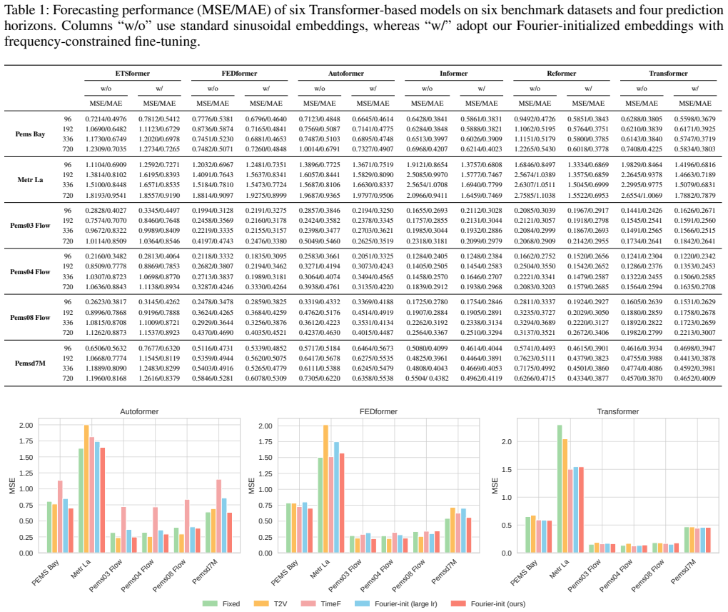
On its own terms, the paper's central discovery is that spectral bias in learned time embeddings—trained frequencies drifting toward sharp high-frequency basins—can be countered by combining a data-driven frequency prior with a constrained optimization schedule. The method (i) solves a non-convex harmonic decomposition by FFT-guided coordinate descent, replacing direct gradient descent on frequencies; (ii) uses the recovered $\{\omega_k\}$ to initialize a Time2Vec-style sinusoidal embedding $\phi(t)=\bigoplus_{k=1}^K[\cos(\omega_k t+b_k),\sin(\omega_k t+b_k)]$; and (iii) updates $\{\omega_k\}$ with a learning rate of $10^{-5}$ while all other parameters use $10^{-3}$. The empirical claim is that this pairing, and only this pairing, consistently improves long-term forecasting: on PEMS03, Autoformer's horizon-720 MSE falls from 0.5049 to 0.2625, and on METR-LA the vanilla Transformer's horizon-720 MSE falls from 2.6554 to 1.7882.
Load-bearing premise
The method assumes the dominant periodicities found in the 2016-step lookback window are the same periodicities that govern the forecast horizon (up to 720 steps ahead), so pinning the learned frequencies near the FFT initialization helps instead of locking the model onto outdated cycles.
Editorial extensions
If this is right
- Replacing standard sinusoidal or learnable time embeddings with the Fourier-initialized, frequency-constrained embedding lowers MSE/MAE on all six Transformer backbones and all six traffic datasets, with the largest relative gains at horizons 336 and 720.
- On PEMS03, Autoformer's horizon-720 MSE drops from 0.5049 to 0.2625; on METR-LA, the vanilla Transformer's horizon-720 MSE drops from 2.6554 to 1.7882, showing the gain is not limited to strongly periodic data.
- The synthetic experiments show FFT initialization with a small frequency learning rate reaches a low-frequency hit rate of 1.00, while random initialization or large frequency learning rates settle near spurious high frequencies, with hit rates between 0.22 and 0.31.
- Ablations imply the two ingredients are complementary: FFT initialization without the constrained learning rate, or the constrained rate without spectral initialization, both underperform the full method.
- Because the embedding is a drop-in module with no backbone modifications, the claimed gains apply to any Transformer-based forecaster that uses sinusoidal or learnable time embeddings.
Reading between the lines
- We infer a testable extension is to re-extract or adapt frequencies per sliding window, or to raise the frequency learning rate over time, so the method can track drifting periodicities; the paper's stationarity assumption suggests this is where the current design would strain.
- We infer the same embedding would help in other domains with strong stationary seasonality, such as energy load, retail demand, or climate indices, since the mechanism is domain-agnostic; the paper only demonstrates traffic.
- We infer the learned $\omega_k$ values could be read as interpretable seasonal periods, giving practitioners a direct explanation of which cycles the forecast relies on.
- We infer the two-speed schedule suggests a broader design principle: spectral parameters in deep models should be seeded from data-driven priors and updated with smaller steps than the rest of the network, a principle that could extend to other Fourier or wavelet modules.
Editorial analysis
A structured set of objections, weighed in public.
Referee Report
Summary. The paper proposes a model-agnostic periodic time embedding for Transformer-based long-term forecasting. Frequencies are extracted from the training signal by FFT-guided coordinate descent, embedded through a sinusoidal Time2Vec-style basis, and then trained with a reduced learning rate so that they stay close to their spectral initialization. The authors claim consistent performance improvements across six Transformer backbones and six traffic datasets, and accurate recovery of ground-truth frequencies on a synthetic multi-frequency signal. The main text presents a table of MSE/MAE results, ablations against other time embeddings, and a synthetic experiment with four initialization/learning-rate combinations.
Significance. If the claims were true, the method would offer a simple, interpretable, drop-in replacement for the time embedding in existing Transformer forecasting models, with potential practical value for long-horizon periodic data. The method's motivation—that unconstrained frequency learning drifts toward high-frequency basins—is plausible and connects to a real literature on spectral bias. However, the central empirical claim is contradicted by the paper's own Table 1, and the synthetic validation is largely predetermined by the initialization combined with a tiny frequency learning rate. As presented, the contribution is not established, and the inconsistent implementation details further reduce confidence in the reported experiments.
major comments (5)
- [Section 4 (Main Results), Table 1] The claim that the Fourier-initialized embedding "consistently improves long-term forecasting performance across all six Transformer-based backbones and datasets" is directly contradicted by Table 1. ETSformer with the proposed embedding is worse than the baseline in all 24 dataset-horizon cells; for example, on PEMS Bay at horizon 96 the MSE degrades from 0.7214 to 0.7812, on METR-LA at horizon 96 from 1.1104 to 1.2592, and on PEMS03 at horizon 96 from 0.2828 to 0.3345. FEDformer is worse at all four horizons on METR-LA, and Autoformer is worse at METR-LA horizons 336 and 720. The conclusion should be revised to describe which backbones and datasets actually benefit, or the experiments must be corrected, before the central "consistent improvement" claim can stand.
- [Section 4 (Implementation Details), Table 1] All results are reported as 5-run averages with no standard deviations, confidence intervals, or paired significance tests. Without these, the favorable cells for Informer and Reformer cannot be distinguished from run-to-run noise, while the ETSformer degradations are systematic across all 24 cells. The paper should provide per-cell variance estimates and a paired test (e.g., across seeds or across datasets) to support any claim of consistent, statistically meaningful improvement.
- [Section 4.2 (Synthetic Experiments), Figure 2] The synthetic frequency-recovery result for "FFT x Small LR" is essentially determined by the initialization. With ηω = 1e-6 over 2,000 Adam steps, the frequency parameters move by an almost negligible amount, and the reported Phit = 1.00 with tolerance δ = 0.005 measures the FFT initialization, not a learned recovery. To support the interpretability claim, the paper should report the initial versus final frequencies, include a control that freezes the FFT-initialized frequencies, or use a larger frequency learning rate and show that the frequencies still converge to the true low-frequency modes.
- [Conclusion, last paragraph] The paper acknowledges in the Conclusion that the method "assumes the dominant periodicities are stationary and globally shared across training windows." This assumption is load-bearing because the frequencies are extracted from a 2016-point Fourier window (Table 5) and then kept nearly fixed while forecasting up to 720 steps ahead. The synthetic experiment uses stationary sinusoids and therefore cannot test whether the method adapts to spectral drift or to differences between the lookback window and the target horizon. The paper should either add nonstationary or drifting-frequency experiments or explicitly restrict the claims to stationary periodic settings.
- [Section 3.2 (Periodic Embedding via Time2Vec) and Section 4 (Implementation Details)] There is an architectural inconsistency in the embedding dimension. Section 3.2 states that dmodel = 2K for the periodic embedding, but Table 5 fixes K = 10 and Section 4 states the embedding dimension is 512 across all models. Since the final embedding is ht = ValueEmbed(xt) + PosEmbed(t) + PeriodEmbed(t), the dimensions must match; the text should clarify whether a linear projection maps the 20-dimensional periodic embedding to 512, or whether K is set differently in the real experiments.
minor comments (4)
- [Section 3.3, Eq. (9)] Equation (9) contains a sign typo: it reads "ωk ← −ωk − ηω ∇ωk L", which would make the frequency update diverge; the intended update is presumably "ωk ← ωk − ηω ∇ωk L".
- [Tables 1 and 6/7] Dataset names are inconsistent: the text refers to PEMS07 while Table 1 labels it "Pemsd7M", and "Metr La" appears alongside "METR-LA" in different places. Please unify the naming.
- [Supplementary Material, Tables 6 and 7] Tables 6 and 7 appear to report the same ablation results with the same structure; one of them should be removed or the two should be clearly differentiated (e.g., one for MSE/MAE by horizon and one for horizon-averaged values).
- [Figure 2(b)] The y-axis label "Learned frequency k" is ambiguous; it should be labeled as frequency ωk or f with units, and the figure should clarify that each row of points corresponds to one of the 10 runs.
Circularity Check
Synthetic frequency 'recovery' is predetermined by the FFT initialization under the 1e-6 frequency learning rate; the real forecasting benchmarks remain external and non-circular.
-
fitted input called prediction
[Synthetic Experiments, Experimental Setup and Results (Figure 2)]
"FFT init initialize {ωk} to the top K spectral peaks extracted by an FFT of y(t) ... Small LR/Large LR: learning rate for ωk is 10−6/10−3 ... FFT × Small LR achieves Phit = 1.00 and a tight distribution around true low frequencies."
With frequency learning rate ηω = 1e-6 and 2,000 Adam steps, each frequency can move by at most roughly 2e-3 even under idealized unit normalized gradients, which is inside the Phit tolerance δ = 0.005. Therefore the reported final ωk remain within tolerance of the top-K FFT peaks used as initialization. Those peaks are computed from the same y(t) whose generating frequencies define the Phit target, so Phit = 1.00 is forced by the initialization rather than by learned discovery. The paper's own rationale for the schedule confirms this: the constrained update keeps frequencies close to the FFT-guided initialization.
full rationale
The only clear circular reduction in the paper is the synthetic frequency-recovery experiment: the learned frequencies are held within a tiny neighborhood of the FFT-initialized peaks by the two-speed schedule (ηω = 1e-6 over 2,000 steps), and Phit = 1.00 is therefore a measure of the initialization, not of the learning process. This is a fitted input being presented as a recovered prediction. The real-data forecasting comparisons, by contrast, are external benchmarks (PEMS-BAY, METR-LA, PEMS03/04/07/08) evaluated on held-out test sets, so the main forecasting claim has independent content. The self-citations in the paper (Zheng, Choi, and Sun 2025; Kong et al. 2025) are contextual and not load-bearing for the method's derivation. One important caveat is not circularity but correctness: Table 1 directly contradicts the headline claim of 'consistent improvements across all six Transformer-based backbones,' since ETSformer degrades in all 24 reported dataset-horizon cells. That inconsistency, and the absence of significance tests around 5-run averages, should appear in a correctness assessment rather than as a circularity charge. Overall, the central forecasting derivation is self-contained, but the key interpretability validation reduces by construction to its own initialization, giving a partial circularity score of 6.
Assumptions & free parameters
free parameters (4)
- K (number of sinusoidal components) =
k=10 in Table 5, but d_model=512 implies K=256
- Frequency learning rate eta_omega =
1e-5 (real data), 1e-6 (synthetic)
- Fourier init length =
2016
- Coordinate descent tolerance epsilon =
not specified
assumptions (3)
- domain assumption Neural networks suffer from spectral bias toward high-frequency components, causing time embeddings to drift to spurious high frequencies.
- domain assumption Dominant periodicities are stationary and globally shared across training windows.
- domain assumption The additive embedding decomposition (Value + Pos + Period) preserves the model's ability to fuse the periodic prior.
Cite this review
Pith. "Pith review of Frequency-Constrained Learning for Long-Term Forecasting." pith.science (2026). https://pith.science/paper/ZHJZFWIF
@misc{pith2026250801508,
  author       = {Pith},
  title        = {Pith review of: Frequency-Constrained Learning for Long-Term Forecasting},
  year         = {2026},
  howpublished = {\url{https://pith.science/paper/ZHJZFWIF}},
  note         = {Machine review of arXiv:2508.01508}
}
read the original abstract
Many real-world time series exhibit strong periodic structures arising from physical laws, human routines, or seasonal cycles. However, modern deep forecasting models often fail to capture these recurring patterns due to spectral bias and a lack of frequency-aware inductive priors. Motivated by this gap, we propose a simple yet effective method that enhances long-term forecasting by explicitly modeling periodicity through spectral initialization and frequency-constrained optimization. Specifically, we extract dominant low-frequency components via Fast Fourier Transform (FFT)-guided coordinate descent, initialize sinusoidal embeddings with these components, and employ a two-speed learning schedule to preserve meaningful frequency structure during training. Our approach is model-agnostic and integrates seamlessly into existing Transformer-based architectures. Extensive experiments across diverse real-world benchmarks demonstrate consistent performance gains--particularly at long horizons--highlighting the benefits of injecting spectral priors into deep temporal models for robust and interpretable long-range forecasting. Moreover, on synthetic data, our method accurately recovers ground-truth frequencies, further validating its interpretability and effectiveness in capturing latent periodic patterns.
Figures


Reference graph
Works this paper leans on
-
[1]
, " * write output.state after.block = add.period write newline
ENTRY address archivePrefix author booktitle chapter edition editor eid eprint howpublished institution isbn journal key month note number organization pages publisher school series title type volume year label extra.label sort.label short.list INTEGERS output.state before.all mid.sentence after.sentence after.block FUNCTION init.state.consts #0 'before.a...
-
[2]
write newline
" write newline "" before.all 'output.state := FUNCTION n.dashify 't := "" t empty not t #1 #1 substring "-" = t #1 #2 substring "--" = not "--" * t #2 global.max substring 't := t #1 #1 substring "-" = "-" * t #2 global.max substring 't := while if t #1 #1 substring * t #2 global.max substring 't := if while FUNCTION word.in bbl.in capitalize " " * FUNCT...
-
[3]
Berk, K. N. 1974. Consistent autoregressive spectral estimates. The Annals of Statistics, 489--502
work page 1974
-
[4]
Brunton, S. L.; Proctor, J. L.; and Kutz, J. N. 2016. Koopman Invariant Subspaces and Finite‐Dimensional Linear Representations of Nonlinear Dynamical Systems for Control. PLOS ONE, 11(2): e0150171
work page 2016
-
[5]
Cleveland, R. B.; Cleveland, W. S.; McRae, J. E.; and Terpenning, I. 1990. STL: A seasonal-trend decomposition procedure based on loess. Journal of Official Statistics, 6(1): 3--73
work page 1990
-
[6]
Crabb \'e , J.; Huynh, N.; Stanczuk, J.; and Van Der Schaar, M. 2024. Time series diffusion in the frequency domain. arXiv preprint arXiv:2402.05933
arXiv 2024
-
[7]
Dette, H.; and Melas, V. B. 2003. Optimal designs for estimating individual coefficients in Fourier regression models. The Annals of Statistics, 31(5): 1669--1692
work page 2003
-
[8]
Fu, K.; Li, H.; and Shi, X. 2024. An encoder--decoder architecture with Fourier attention for chaotic time series multi-step prediction. Applied Soft Computing, 156: 111409
work page 2024
Show all 35 references
-
[9]
V.; Gehrke, J.; Labrinidis, A.; Papakonstantinou, Y.; Patel, J
Jagadish, H. V.; Gehrke, J.; Labrinidis, A.; Papakonstantinou, Y.; Patel, J. M.; Ramakrishnan, R.; and Shahabi, C. 2014. Big Data and Its Technical Challenges. In Communications of the ACM, volume 57, 86--94
2014
-
[10]
Y.; Shi, X.; Chen, P.-Y.; Liang, Y.; Li, Y.-F.; Pan, S.; et al
Jin, M.; Wang, S.; Ma, L.; Chu, Z.; Zhang, J. Y.; Shi, X.; Chen, P.-Y.; Liang, Y.; Li, Y.-F.; Pan, S.; et al. 2023. Time-llm: Time series forecasting by reprogramming large language models. arXiv preprint arXiv:2310.01728
2023 arXiv
-
[11]
M.; Goel, R.; Eghbali, S.; Ramanan, J.; Sahota, J.; Thakur, S.; Wu, S.; Smyth, C.; Poupart, P.; and Brubaker, M
Kazemi, S. M.; Goel, R.; Eghbali, S.; Ramanan, J.; Sahota, J.; Thakur, S.; Wu, S.; Smyth, C.; Poupart, P.; and Brubaker, M. 2019. Time2vec: Learning a vector representation of time. arXiv preprint arXiv:1907.05321
2019 arXiv
-
[12]
Kitaev, N.; Kaiser, L.; and Levskaya, A. 2020. Reformer: The Efficient Transformer. In International Conference on Learning Representations (ICLR)
2020
-
[13]
Z.; Wang, X.; and Sun, L
Kong, M.; Zheng, V. Z.; Wang, X.; and Sun, L. 2025. Dynamic Modes as Time Representation for Spatiotemporal Forecasting. arXiv preprint arXiv:2506.01212
2025 arXiv
-
[14]
L.; and Kutz, J
Lange, H.; Brunton, S. L.; and Kutz, J. N. 2021. From Fourier to Koopman: Spectral Methods for Long‐term Time Series Prediction. Journal of Machine Learning Research, 22(196): 1--38
2021
-
[15]
Li, Y.; Yu, R.; Shahabi, C.; and Liu, Y. 2018. Diffusion Convolutional Recurrent Neural Network: Data-Driven Traffic Forecasting. In International Conference on Learning Representations (ICLR)
2018
-
[16]
Lin, S.; Lin, W.; Hu, X.; Wu, W.; Mo, R.; and Zhong, H. 2024. Cyclenet: Enhancing time series forecasting through modeling periodic patterns. Advances in Neural Information Processing Systems, 37: 106315--106345
2024
-
[17]
Liu, Y.; Wu, H.; Wang, J.; and Long, M. 2022. Non-stationary transformers: Exploring the stationarity in time series forecasting. Advances in neural information processing systems, 35: 9881--9893
2022
-
[18]
Lotfipoor, A.; Patidar, S.; and Jenkins, D. P. 2024. Deep neural network with empirical mode decomposition and Bayesian optimisation for residential load forecasting. Expert systems with applications, 237: 121355
2024
-
[19]
P.; van Straaten, C.; O, S.; Mamalakis, A.; Cavicchia, L.; Coumou, D.; de Luca, P.; Kretschmer, M.; and Donat, M
Materia, S.; Garc \' a, L. P.; van Straaten, C.; O, S.; Mamalakis, A.; Cavicchia, L.; Coumou, D.; de Luca, P.; Kretschmer, M.; and Donat, M. 2024. Artificial intelligence for climate prediction of extremes: State of the art, challenges, and future perspectives. Wiley Interdisc...
2024
-
[20]
Rahaman, N.; Baratin, A.; Arpit, D.; Draxler, F.; Lin, M.; Hamprecht, F.; Bengio, Y.; and Courville, A. 2019. On the spectral bias of neural networks. In International conference on machine learning, 5301--5310. PMLR
2019
-
[21]
Rao, R.; Bhattacharya, N.; Thomas, N.; Duan, Y.; Chen, X.; Canny, J.; Abbeel, P.; and Song, Y. S. 2019. Evaluating protein transfer learning with TAPE. In Advances in Neural Information Processing Systems, volume 32
2019
-
[22]
Shaw, P.; Uszkoreit, J.; and Vaswani, A. 2018. Self-attention with relative position representations. arXiv preprint arXiv:1803.02155
2018 arXiv
-
[23]
H.; and Stoffer, D
Shumway, R. H.; and Stoffer, D. S. 2000. Time series analysis and its applications, volume 3. Springer
2000
-
[24]
Su, J.; Ahmed, M.; Lu, Y.; Pan, S.; Bo, W.; and Liu, Y. 2024. Roformer: Enhanced transformer with rotary position embedding. Neurocomputing, 568: 127063
2024
-
[25]
Tancik, M.; Srinivasan, P.; Mildenhall, B.; Fridovich-Keil, S.; Raghavan, N.; Singhal, U.; Ramamoorthi, R.; Barron, J.; and Ng, R. 2020. Fourier features let networks learn high frequency functions in low dimensional domains. Advances in neural information processing systems, ...
2020
-
[26]
N.; Kaiser, L.; and Polosukhin, I
Vaswani, A.; Shazeer, N.; Parmar, N.; Uszkoreit, J.; Jones, L.; Gomez, A. N.; Kaiser, L.; and Polosukhin, I. 2017. Attention is all you need. In Advances in neural information processing systems, 5998--6008
2017
-
[27]
Wen, Q.; Gao, J.; Song, X.; Sun, L.; Xu, H.; and Zhu, S. 2019. RobustSTL: A robust seasonal-trend decomposition algorithm for long time series. In Proceedings of the AAAI conference on artificial intelligence, volume 33, 5409--5416
2019
-
[28]
Woo, G.; Liu, C.; Sahoo, D.; Kumar, A.; and Hoi, S. 2022. Etsformer: Exponential smoothing transformers for time-series forecasting. arXiv preprint arXiv:2202.01381
2022 arXiv
-
[29]
Wu, H.; Hu, T.; Liu, Y.; Zhou, H.; Wang, J.; and Long, M. 2022. Timesnet: Temporal 2d-variation modeling for general time series analysis. arXiv preprint arXiv:2210.02186
2022 arXiv
-
[30]
Wu, H.; Xu, J.; Wang, J.; and Long, M. 2021. Autoformer: Decomposition transformers with auto-correlation for long-term series forecasting. Advances in neural information processing systems, 34: 22419--22430
2021
-
[31]
Zeng, A.; Chen, M.; Zhang, L.; and Xu, Q. 2023. Are transformers effective for time series forecasting? In Proceedings of the AAAI conference on artificial intelligence, volume 37, 11121--11128
2023
-
[32]
Zhang, J.; Zheng, Y.; and Qi, D. 2017. Deep Spatio-Temporal Residual Networks for Citywide Crowd Flows Prediction. In AAAI, 1655--1661
2017
-
[33]
Z.; Choi, S.; and Sun, L
Zheng, V. Z.; Choi, S.; and Sun, L. 2025. Probabilistic Traffic Forecasting with Dynamic Regression. Transportation Science
2025
-
[34]
Zhou, H.; Zhang, S.; Peng, J.; Zhang, S.; Li, J.; Xiong, H.; and Zhang, W. 2021. Informer: Beyond efficient transformer for long sequence time-series forecasting. In Proceedings of the AAAI Conference on Artificial Intelligence, volume 35, 11106--11115
2021
-
[35]
Zhou, T.; Ma, Z.; Wen, Q.; Zhou, X.; Yang, W.; Wang, L.; and Wang, W. 2022. Fedformer: Frequency enhanced decomposed transformer for long-term series forecasting. In International Conference on Machine Learning, 27392--27402. PMLR
2022
Reviewed August 6, 2026 · model on record in the stance chip above.
Discussion (0). Sign in to comment.