REVIEW 3 major objections 5 minor 73 references
Four exact power-law Bianchi type I solution families exist for a scalar coupled to three vector fields; stability selects the survivors by relative coupling strength.
Reviewed by Pith at T0; open to challenge. T0 means a machine referee read the full paper against a public rubric. the ladder, T0–T4 →
T0 review · deepseek-v4-flash
2026-08-03 21:27 UTC pith:7OWZ4B7D
load-bearing objection A useful classification of multi-vector Bianchi I power-law solutions with a real stability gap: the existence part is solid, the type II/III stability regions are inferred by visual matching, not derived. the 3 major comments →
Power-law Bianchi type I inflation with multiple vector fields
The pith
A machine-rendered reading of the paper's core claim, the machinery that carries it, and where it could break.
Core claim
The authors claim that in the considered model there exist exactly four power-law solution families — type 0 with no vector fields, type I with one, type II with two, and type III with three — and that each solution is stable against homogeneous perturbations precisely in its specified stability region. The stability conditions are given quantitatively as simple inequalities involving the scalar exponent λ and the coupling exponents ρa, ρb, ρc, and qualitatively: for stability, the surviving fields' couplings must be sufficiently large and, when several survive, sufficiently close to one another, while the suppressed fields' couplings must be significantly smaller. The authors further claim
What carries the argument
The analysis rests on the six-variable autonomous dynamical system built from the anisotropy variables Xb, Xc, the scalar-velocity ratio Y, and the three normalized vector-field amplitudes Za, Zb, Zc, with α (logarithm of the scale factor) as the time coordinate. Fixed points of this system correspond one-to-one to the power-law solutions, and linearization around each fixed point plus a classical root-location criterion on the perturbation matrix yields the stability regions. The qualitative selection rule emerges from comparing these regions: the inequalities encode that a vector field survives exactly when its coupling exponent dominates the others sufficiently.
Load-bearing premise
The load-bearing premise is that the simple inequalities describing stability of the two-vector and three-vector solutions exactly match the full mathematical stability conditions — the paper says it tries to guess this equivalence from plots rather than proving it, and if the guess is off, the claimed stability of these solutions in the tabulated regions is unsupported.
What would settle it
Take λ=1.5 and (ρa,ρb,ρc)=(1,1,1), which lies in the claimed stability region for the three-vector fixed point. Substitute the fixed point into the 6x6 perturbation matrix of the autonomous system and compute the eigenvalues. If any eigenvalue has real part ≥0, the claimed identity between the stability region and the existence region fails. A more systematic check: evaluate the full stability determinants at several points just inside the claimed boundaries of the type III and type IIbc regions and compare their signs with the simple inequalities; one sign mismatch is a counterexample.
If this is right
- If the classification is right, the final state of an anisotropic inflationary universe is determined by which gauge-coupling exponents are largest; all other initial data wash out.
- The cosmic no-hair conjecture is violated when at least one coupling is large enough: anisotropies and vector fields persist, and the metric settles to a Bianchi type I (or LRS) power-law form rather than FLRW.
- When all couplings are small, the standard isotropic FLRW power-law inflation is the attractor, consistent with cosmic no-hair.
- The magnitude of the spatial anisotropies depends on the number of surviving vector fields: three or two surviving fields give general Bianchi I anisotropy, one gives LRS Bianchi I, none gives FLRW.
- The same power-law framework and stability analysis can be used to compute observable signatures, since the authors note CMB imprints are left for future work.
Where Pith is reading between the lines
- The selection rule is stated for three vector fields; by symmetry of the autonomous system, a plausible extension is that with N vectors, the survivors are exactly those whose coupling exponents exceed the others by a threshold set by λ — a testable extension for N > 3.
- The stability boundaries bracket the regime where the vector-field energy and anisotropy approach their attractor values extremely slowly; such slow approach could lengthen or shorten inflation in a parameter-dependent way, which may be observable in the spectral tilt if the model is coupled to perturbations.
- Since the paper only considers positive coupling exponents and a positive scalar exponent, the classification might extend to negative couplings, which correspond to suppressed gauge kinetic functions; whether the selection rule inverts there is an open extension.
- The paper's guessed equality between simplified and full stability regions could be turned into a rigorous algebraic proof by showing the stability determinants factorize on the existence region; that would pin the boundaries exactly.
Editorial analysis
A structured set of objections, weighed in public.
Referee Report
Summary. The paper studies a supergravity-motivated model in which a single scalar field with exponential potential V(ϕ)=V0 e^{λϕ} is non-minimally coupled, through exponential gauge kinetic functions f_i(ϕ)=f_{i0} e^{ρ_i ϕ}, to three vector fields aligned along the three spatial axes of a general Bianchi type I metric. Using the power-law ansatz α=ζ log t, σ_b=η_b log t, σ_c=η_c log t, ϕ=ξ log t+φ0, the field equations are reduced to algebraic systems. The authors find exact power-law solutions of four types — type 0 (no vector fields), type I a/b/c (one vector field), type II ab/ac/bc (two vector fields), and type III (three vector fields) — summarized in Table I. They then construct a six-dimensional autonomous system in variables (X_b, X_c, Y, Z_a, Z_b, Z_c), identify the corresponding fixed points, and use linearization and the Routh–Hurwitz criterion to claim stability regions for each fixed point, summarized in Table II and Eqs. (4.27)–(4.33). They also claim a qualitative selection rule: for fixed λ, if all coupling constants are sufficiently small the vector fields are diluted; if at least one is sufficiently large, the vector field(s) with the largest and sufficiently close couplings persist, determining the late-time metric. Numerical integration in Sec. IV G is presented as confirmation.
Significance. If the results are correct, the paper provides a useful and fairly systematic extension of the Kanno–Soda–Watanabe anisotropic inflation model to multiple vector fields in a general Bianchi type I spacetime. The existence part of the derivation is a transparent algebraic exercise: substituting the ansatz reduces the field equations to polynomial systems, and the resulting solutions are internally consistent as far as the text shows. The paper also has clear strengths: explicit formulas for the solutions and fixed points, factorized eigenvalue equations for types 0 and I, a concrete and falsifiable qualitative selection rule, and numerical demonstrations of attractor behavior for representative parameter points. However, the central quantitative claim — that all solutions are stable under exactly the tabulated conditions — is not fully established for types II and III, because the stability regions there are identified by visual inspection of Routh–Hurwitz plots rather than by a complete algebraic derivation. This gap is load-bearing for Table II and for the qualitative selection rule in Sec. IV F. If the missing verification is supplied, the paper would be a solid contribution to t
major comments (3)
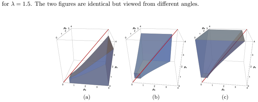
- [Appendix B, Eq. (B11) and Fig. 12] The stability region for the type IIbc fixed point is not derived. The text states that the Routh–Hurwitz condition for the quartic factor is 'very cumbersome' and that the authors 'plot the unsimplified stability region according to the Routh–Hurwitz criterion in parameter space and try to guess its simplified version by comparing it to the existence region.' The subsequent claim that the quartic condition (B13) is exactly the existence region (4.18) is therefore an inference from plots, not a proof. This equivalence is used to obtain the stability region (4.28) and feeds directly into the qualitative claims in Sec. IV F and Table II. Please provide an explicit algebraic verification of this equivalence (e.g., the full Hurwitz determinants, or a computer-algebra quantifier-elimination certificate).
- [Sec. IV F and Appendix B, Fig. 13] The same issue occurs for fixed point type III. The degree-6 eigenvalue polynomial is not written out, and the claimed equality between the stability region and the existence region (4.24) is inferred from plots for λ=1.5 and 'other values of λ.' This does not establish the abstract's claim that all solutions are stable under the tabulated conditions. Since the Routh–Hurwitz criterion is a finite algebraic condition, an exact verification should be possible; at minimum, the polynomial and the resulting reduced inequality set should be supplied, or a rigorous proof that (4.24) is both necessary and sufficient for all positive λ, ρ_a, ρ_b, ρ_c.
- [Sec. IV G] The numerical checks sample one point well inside each claimed stability region (e.g., Eqs. (4.35)–(4.37)). They do not probe the boundaries of the regions or test the claimed exact identity between the Routh–Hurwitz region and the simplified inequalities for types IIbc and III. Thus the numerics are consistent with the stability claims but do not resolve the unproven equivalence identified above.
minor comments (5)
- [Eq. (3.4)] The third anisotropy is written as X_c = η_b/ζ; it should be X_c = η_c/ζ.
- [Eq. (3.13)] In the last formula of the type Ic solution, ω_b should presumably be ω_c. Please check analogous relabelings in the type II formulas.
- [Sec. IV D] 'we will it the fixed point type II bc' should read 'we call it the fixed point type II bc.'
- [Fig. 12 caption] 'Notte' should be 'Note.'
- [Notation throughout Sec. IV] The notation alternates between (Za)^2, (Z_a)^2, and Z_a^2. Please use a single uniform notation, e.g., Z_a^2.
Circularity Check
No significant circularity; the derivation is self-contained, with only an unproven (but non-circular) visual inference in Appendix B simplifying some stability regions.
full rationale
The paper's central chain is: action (2.9) → field equations → power-law ansatz → algebraic solutions of types 0, I, II, III → autonomous dynamical system → fixed points → stability via eigenvalues/Routh–Hurwitz. No parameter is fitted to any target result, and the exponential potential and gauge kinetic functions are model inputs from the KSW program, not outputs of the analysis. The type 0 and type I stability eigenvalue equations are factorized explicitly in Appendix B, so those stability regions are genuinely derived. For type IIbc and type III, the paper admits in Appendix B that it plots the unsimplified Routh–Hurwitz stability region and 'try to guess its simplified version by comparing it to the existence region' (type IIbc), and 'plot its stability region' and conclude equality with Eq. (4.24)' (type III). This is an unsupported inference and a proof gap, but it is not circular: the plotted region is generated by the Routh–Hurwitz criterion itself, not by the simplified inequalities, and no fitted data or self-citation is used to force the result. The numerical checks sample interior points and therefore do not independently verify the boundary equivalence, but they are consistency tests rather than fitted predictions. The paper's self-citations are contextual and not load-bearing, and no uniqueness theorem is imported from the authors' prior work. Overall, no step reduces by construction to its own input; the appropriate finding is no significant circularity, with the Appendix B inferred equivalences noted as a correctness risk rather than a circularity.
Axiom & Free-Parameter Ledger
free parameters (4)
- lambda
- rho_a
- rho_b
- rho_c
axioms (7)
- domain assumption Bianchi type I metric with three independent scale factors (2.1)-(2.2)
- domain assumption Field configuration of one homogeneous scalar and three mutually orthogonal vector fields (2.13)
- domain assumption Exponential potential and gauge kinetic functions V=V0 exp(lambda*phi), f_i=f_i0 exp(rho_i*phi) (3.1)
- ad hoc to paper Power-law ansatz alpha=zeta log t, sigma_b=eta_b log t, sigma_c=eta_c log t, phi=xi log t+phi0 (3.2)
- domain assumption Positivity of the potential, Eq. (4.8)
- domain assumption All parameters lambda, rho_a, rho_b, rho_c are positive
- standard math Routh-Hurwitz criterion
read the original abstract
We investigate an inflationary anisotropic universe in a supergravity-motivated model with one scalar field non-minimally coupled to multiple vector fields. We restrict ourselves to the Bianchi type I metric, which describes a homogeneous but anisotropic universe. For consistency, we consider a configuration consisting of one homogeneous scalar field and three mutually orthogonal vector fields. As a result, we find four types of power-law solutions, classified according to the number of non-vanishing vector fields. Moreover, we show that all these solutions are stable under certain conditions on the model parameters, thereby defining stability regions described both quantitatively and qualitatively. Interestingly, our analysis suggests that vector fields with significantly larger coupling constants tend to persist as the universe expands, while those with significantly smaller coupling constants are eventually diluted. On the other hand, we also find that the anisotropies depend on the number of persisting vector fields. Furthermore, our claims are confirmed by numerical calculations. This work may therefore shed light on how vector fields and anisotropies evolve in an inflationary universe.
Figures




Reference graph
Works this paper leans on
-
[1]
This means that it corresponds to a power-law FLR W metric, ds2 =−dt 2 +t 4/λ2 (dx2 +dy 2 +dz 2),(3.9) where the scale factorsa(t) =b(t) =c(t) =t 2/λ2
We notice thatη a =η b =η c = 0 for this solution. This means that it corresponds to a power-law FLR W metric, ds2 =−dt 2 +t 4/λ2 (dx2 +dy 2 +dz 2),(3.9) where the scale factorsa(t) =b(t) =c(t) =t 2/λ2 . This type of solution can be found in Ref. [29]. B. Solutions type I In a case whereA µ is the only non-vanishing vector field, i.e.,p a ̸= 0 andp b =p c...
-
[2]
(4.27) For a fixedλ, the stability region is a cube bounded by three planes:ρ a = (4−λ 2)/(2λ),ρ b = (4−λ 2)/(2λ), and ρc = (4−λ 2)/(2λ)
Fixed point type 0 The stability region of the fixed point type 0 is determined by the following inequalities, λ2 + 2λρa −4<0, λ 2 + 2λρb −4<0, λ 2 + 2λρc −4<0. (4.27) For a fixedλ, the stability region is a cube bounded by three planes:ρ a = (4−λ 2)/(2λ),ρ b = (4−λ 2)/(2λ), and ρc = (4−λ 2)/(2λ). Qualitatively, in order to make the fixed point type 0 sta...
-
[3]
The ex- istence region of the fixed point type III is determined by three inequalities shown in Eq
Fixed point type III Contrast to the fixed point type 0, which clearly isotropic, the fixed point type III is generically anisotropic. The ex- istence region of the fixed point type III is determined by three inequalities shown in Eq. (4.24) and depicted as a dark blue region forλ= 1.5 in Fig. 2. This region is bounded by three surfaces:−4+λ 2 +2λρa −4 ρ2...
-
[4]
Its existence region, determined by Eq
Fixed points type II Let us continue with the fixed point type IIbc. Its existence region, determined by Eq. (4.18), is depicted in Fig. 3a as the orange one, which is bounded by two surfaces:−4+λ(λ+2ρ b)−4ρ c(ρc−ρb) = 0 and−4+λ(λ+2ρ c)−4ρ b(ρb−ρc) =
-
[5]
(4.28) It is apparent that this region differs from the existence region by the additional third inequality
However, the stability region of this fixed point must follow the corresponding inequalities, −4 +λ 2 + 2λρb −4ρ c(ρc −ρ b)>0, −4 +λ 2 + 2λρc −4ρ b(ρb −ρ c)>0, −4 +λ 2 + 2λρa −4 ρ2 b +ρ 2 c −ρ a(ρb +ρ c) <0. (4.28) It is apparent that this region differs from the existence region by the additional third inequality. To be more specific, this stability regi...
-
[6]
Fixed points type I In the next step, we would like to combine the stability regions of the fixed points found above into one figure to form athree-bladed turbine-shaperegion (see Fig. 5). The cube at the corner, the turbine shaft and turbine blades are the stability regions of the fixed points type 0, III, II bc, II ac, and II ab respectively. One might ...
2023
-
[7]
P. K. Aluri, P. Cea, P. Chingangbam, M. C. Chu, R. G. Clowes, D. Hutsem´ ekers, J. P. Kochappan, A. M. Lopez, L. Liu, and N. C. M. Martens,et al.Class. Quant. Grav.40, no.9, 094001 (2023) doi:10.1088/1361-6382/acbefc [arXiv:2207.05765 [astro-ph.CO]]
Pith/arXiv arXiv 2023
-
[8]
G. W. Gibbons and S. W. Hawking, Phys. Rev. D15, 2738-2751 (1977) doi:10.1103/PhysRevD.15.2738
-
[9]
S. W. Hawking and I. G. Moss, Phys. Lett. B110, 35-38 (1982) doi:10.1016/0370-2693(82)90946-7
-
[10]
R. M. Wald, Asymptotic behavior of homogeneous cosmological models in the presence of a positive cosmological constant, Phys. Rev. D28, 2118 (1983)
1983
-
[11]
J. D. Barrow, Cosmic no hair theorems and inflation, Phys. Lett. B187, 12 (1987)
1987
-
[12]
Mijic and J
M. Mijic and J. A. Stein-Schabes, A no-hair theorem forR 2 models, Phys. Lett. B203, 353 (1988)
1988
-
[13]
Kitada and K
Y. Kitada and K. i. Maeda, Cosmic no hair theorem in power law inflation, Phys. Rev. D45, 1416 (1992)
1992
-
[14]
M. Kleban and L. Senatore, Inhomogeneous anisotropic cosmology, J. Cosmol. Astropart. Phys.10(2016) 022 [arXiv:1602.03520]
Pith/arXiv arXiv 2016
-
[15]
W. E. East, M. Kleban, A. Linde, and L. Senatore, Beginning inflation in an inhomogeneous universe, J. Cosmol. Astropart. Phys.09(2016) 010 [arXiv:1511.05143]
Pith/arXiv arXiv 2016
-
[16]
S. M. Carroll and A. Chatwin-Davies, Cosmic equilibration: A holographic no-hair theorem from the generalized second law, Phys. Rev. D97, 046012 (2018) [arXiv:1703.09241]
Pith/arXiv arXiv 2018
-
[17]
Kaloper, Lorentz Chern-Simons terms in Bianchi cosmologies and the cosmic no hair conjecture, Phys
N. Kaloper, Lorentz Chern-Simons terms in Bianchi cosmologies and the cosmic no hair conjecture, Phys. Rev. D44, 2380 (1991)
1991
-
[18]
J. D. Barrow and S. Hervik, Anisotropically inflating universes, Phys. Rev. D73, 023007 (2006) [gr-qc/0511127]
Pith/arXiv arXiv 2006
-
[19]
H. W. H. Tahara, S. Nishi, T. Kobayashi, and J. Yokoyama, Self-anisotropizing inflationary universe in Horndeski theory and beyond, J. Cosmol. Astropart. Phys.07, 058 (2018) [arXiv:1805.00186]
Pith/arXiv arXiv 2018
-
[20]
A. A. Starobinsky, S. V. Sushkov, and M. S. Volkov, Anisotropy screening in Horndeski cosmologies, Phys. Rev. D101, 064039 (2020) [arXiv:1912.12320]
Pith/arXiv arXiv 2020
-
[21]
R. Galeev, R. Muharlyamov, A. A. Starobinsky, S. V. Sushkov, and M. S. Volkov, Anisotropic cosmological models in Horndeski gravity, Phys. Rev. D103, 104015 (2021) [arXiv:2102.10981]
Pith/arXiv arXiv 2021
-
[22]
S. Nojiri, S. D. Odintsov, V. K. Oikonomou, and A. Constantini, Formalizing anisotropic inflation in modified gravity, Nucl. Phys. B985, 116011 (2022) [arXiv:2210.16383]
Pith/arXiv arXiv 2022
-
[23]
A. A. Starobinsky, Isotropization of arbitrary cosmological expansion given an effective cosmological constant, JETP Lett. 37, 66 (1983)
1983
-
[24]
Muller, H
V. Muller, H. J. Schmidt, and A. A. Starobinsky, Power law inflation as an attractor solution for inhomogeneous cosmo- logical models, Class. Quant. Grav.7, 1163 (1990)
1990
-
[25]
J. D. Barrow and J. Stein-Schabes, Inhomogeneous cosmologies with cosmological constant, Phys. Lett. A103, 315 (1984)
1984
-
[26]
L. G. Jensen and J. A. Stein-Schabes, Is inflation natural?, Phys. Rev. D35, 1146 (1987)
1987
-
[27]
J. A. Stein-Schabes, Inflation in spherically symmetric inhomogeneous models, Phys. Rev. D35, 2345 (1987). 26
1987
-
[28]
A. A. Starobinsky, A new type of isotropic cosmological models without singularity, Phys. Lett. B91, 99 (1980)
1980
-
[29]
A. H. Guth, The inflationary universe: A possible solution to the horizon and flatness problems, Phys. Rev. D23, 347 (1981)
1981
-
[30]
A. D. Linde, A new inflationary universe scenario: A possible solution of the horizon, flatness, homogeneity, isotropy and primordial monopole problems, Phys. Lett. B108, 389 (1982)
1982
-
[31]
G. Hinshawet al., Nine-Year Wilkinson Microwave Anisotropy Probe (WMAP) Observations: Cosmological Parameter Results, Astrophys. J. Suppl.208, 19 (2013) [arXiv:1212.5226]
Pith/arXiv arXiv 2013
-
[32]
Y. Akramiet al.[Planck], Astron. Astrophys.641, A7 (2020) doi:10.1051/0004-6361/201935201 [arXiv:1906.02552 [astro- ph.CO]]
Pith/arXiv arXiv 2020
-
[33]
D. J. Schwarz, C. J. Copi, D. Huterer, and G. D. Starkman, Class. Quant. Grav.33, no.18, 184001 (2016) doi:10.1088/0264- 9381/33/18/184001 [arXiv:1510.07929 [astro-ph.CO]]
Pith/arXiv arXiv 2016
-
[34]
M. a. Watanabe, S. Kanno, and J. Soda, Phys. Rev. Lett.102, 191302 (2009) doi:10.1103/PhysRevLett.102.191302 [arXiv:0902.2833 [hep-th]]
Pith/arXiv arXiv 2009
-
[35]
S. Kanno, J. Soda, and M. a. Watanabe, JCAP12, 024 (2010) doi:10.1088/1475-7516/2010/12/024 [arXiv:1010.5307 [hep-th]]
Pith/arXiv arXiv 2010
-
[36]
J. Soda, Class. Quant. Grav.29, 083001 (2012) doi:10.1088/0264-9381/29/8/083001 [arXiv:1201.6434 [hep-th]]
Pith/arXiv arXiv 2012
-
[37]
A. Maleknejad, M. M. Sheikh-Jabbari, and J. Soda, Phys. Rept.528, 161-261 (2013) doi:10.1016/j.physrep.2013.03.003 [arXiv:1212.2921 [hep-th]]
Pith/arXiv arXiv 2013
-
[38]
R. Emami, H. Firouzjahi, S. M. Sadegh Movahed, and M. Zarei, JCAP02, 005 (2011) doi:10.1088/1475-7516/2011/02/005 [arXiv:1010.5495 [astro-ph.CO]]
Pith/arXiv arXiv 2011
-
[39]
K. Murata and J. Soda, JCAP06, 037 (2011) doi:10.1088/1475-7516/2011/06/037 [arXiv:1103.6164 [hep-th]]
Pith/arXiv arXiv 2011
-
[40]
S. Bhowmick and S. Mukherji, Mod. Phys. Lett. A27, 1250009 (2012) doi:10.1142/S0217732312500095 [arXiv:1105.4455 [hep-th]]
Pith/arXiv arXiv 2012
-
[41]
T. Q. Do, W. F. Kao, and I. C. Lin, Phys. Rev. D83, 123002 (2011) doi:10.1103/PhysRevD.83.123002
-
[42]
S. Hervik, D. F. Mota, and M. Thorsrud, JHEP11, 146 (2011) doi:10.1007/JHEP11(2011)146 [arXiv:1109.3456 [gr-qc]]
Pith/arXiv arXiv 2011
-
[43]
T. Q. Do and W. F. Kao, Phys. Rev. D84, 123009 (2011) doi:10.1103/PhysRevD.84.123009
-
[44]
K. Yamamoto, M. a. Watanabe, and J. Soda, Class. Quant. Grav.29, 145008 (2012) doi:10.1088/0264-9381/29/14/145008 [arXiv:1201.5309 [hep-th]]
Pith/arXiv arXiv 2012
-
[45]
K. Yamamoto, Phys. Rev. D85, 123504 (2012) doi:10.1103/PhysRevD.85.123504 [arXiv:1203.1071 [astro-ph.CO]]
Pith/arXiv arXiv 2012
-
[46]
A. Maleknejad and M. M. Sheikh-Jabbari, Phys. Rev. D85, 123508 (2012) doi:10.1103/PhysRevD.85.123508 [arXiv:1203.0219 [hep-th]]
Pith/arXiv arXiv 2012
-
[47]
M. Thorsrud, D. F. Mota, and S. Hervik, JHEP10, 066 (2012) doi:10.1007/JHEP10(2012)066 [arXiv:1205.6261 [hep-th]]
Pith/arXiv arXiv 2012
-
[48]
H. Funakoshi and K. Yamamoto, Class. Quant. Grav.30, 135002 (2013) doi:10.1088/0264-9381/30/13/135002 [arXiv:1212.2615 [astro-ph.CO]]
Pith/arXiv arXiv 2013
-
[49]
J. Ohashi, J. Soda, and S. Tsujikawa, Phys. Rev. D87, no.8, 083520 (2013) doi:10.1103/PhysRevD.87.083520 [arXiv:1303.7340 [astro-ph.CO]]
Pith/arXiv arXiv 2013
-
[50]
J. Ohashi, J. Soda, and S. Tsujikawa, Phys. Rev. D88, 103517 (2013) doi:10.1103/PhysRevD.88.103517 [arXiv:1310.3053 [hep-th]]
Pith/arXiv arXiv 2013
-
[51]
A. Ito and J. Soda, Phys. Rev. D92, no.12, 123533 (2015) doi:10.1103/PhysRevD.92.123533 [arXiv:1506.02450 [hep-th]]
Pith/arXiv arXiv 2015
-
[52]
T. Q. Do and W. F. Kao, Class. Quant. Grav.33, no.8, 085009 (2016) doi:10.1088/0264-9381/33/8/085009
-
[53]
Lahiri, JCAP09, 025 (2016) doi:10.1088/1475-7516/2016/09/025 [arXiv:1605.09247 [hep-th]]
S. Lahiri, JCAP09, 025 (2016) doi:10.1088/1475-7516/2016/09/025 [arXiv:1605.09247 [hep-th]]
Pith/arXiv arXiv 2016
-
[54]
M. Tirandari and K. Saaidi, Nucl. Phys. B925, 403-414 (2017) doi:10.1016/j.nuclphysb.2017.10.017 [arXiv:1701.06890 [gr-qc]]
Pith/arXiv arXiv 2017
-
[55]
T. Q. Do and S. H. Q. Nguyen, Int. J. Mod. Phys. D26, no.07, 1750072 (2017) doi:10.1142/S0218271817500729 [arXiv:1702.08308 [gr-qc]]
Pith/arXiv arXiv 2017
-
[56]
T. Q. Do and W. F. Kao, Phys. Rev. D96, no.2, 023529 (2017) doi:10.1103/PhysRevD.96.023529
-
[57]
A. Ito and J. Soda, Eur. Phys. J. C78, no.1, 55 (2018) doi:10.1140/epjc/s10052-018-5534-5 [arXiv:1710.09701 [hep-th]]
Pith/arXiv arXiv 2018
-
[58]
J. Holland, S. Kanno, and I. Zavala, Phys. Rev. D97, no.10, 103534 (2018) doi:10.1103/PhysRevD.97.103534 [arXiv:1711.07450 [hep-th]]
Pith/arXiv arXiv 2018
-
[59]
T. Q. Do and W. F. Kao, Eur. Phys. J. C78, no.5, 360 (2018) doi:10.1140/epjc/s10052-018-5846-5 [arXiv:1712.03755 [gr-qc]]
Pith/arXiv arXiv 2018
-
[60]
M. Tirandari, K. Saaidi, and A. Mohammadi, Phys. Rev. D98, no.4, 043516 (2018) doi:10.1103/PhysRevD.98.043516
-
[61]
T. Q. Do, Eur. Phys. J. C81, no.1, 77 (2021) doi:10.1140/epjc/s10052-021-08866-7 [arXiv:2007.04867 [gr-qc]]
Pith/arXiv arXiv 2021
-
[62]
M. A. Gorji, S. A. Hosseini Mansoori, and H. Firouzjahi, JCAP11, 041 (2020) doi:10.1088/1475-7516/2020/11/041 [arXiv:2008.08195 [astro-ph.CO]]
Pith/arXiv arXiv 2020
-
[63]
T. Q. Do and W. F. Kao, Eur. Phys. J. C81, no.6, 525 (2021) doi:10.1140/epjc/s10052-021-09334-y [arXiv:2104.14100 [gr-qc]]
Pith/arXiv arXiv 2021
-
[64]
C. B. Chen and J. Soda, JCAP09, 026 (2021) doi:10.1088/1475-7516/2021/09/026 [arXiv:2106.04813 [hep-th]]
Pith/arXiv arXiv 2021
-
[65]
D. H. Nguyen, T. M. Pham, and T. Q. Do, Eur. Phys. J. C81, no.9, 839 (2021) doi:10.1140/epjc/s10052-021-09652-1 [arXiv:2107.14115 [gr-qc]]
Pith/arXiv arXiv 2021
-
[66]
T. Q. Do and W. F. Kao, Eur. Phys. J. C82, 123 (2022) doi:10.1140/epjc/s10052-022-10078-6 [arXiv:2110.13516 [gr-qc]]
Pith/arXiv arXiv 2022
-
[67]
Goodarzi, JCAP11, 052 (2022) doi:10.1088/1475-7516/2022/11/052 [arXiv:2208.10757 [hep-th]]
P. Goodarzi, JCAP11, 052 (2022) doi:10.1088/1475-7516/2022/11/052 [arXiv:2208.10757 [hep-th]]
Pith/arXiv arXiv 2022
-
[68]
S. Kanno, A. Mukuno, J. Soda, and K. Ueda, Phys. Rev. D107, no.6, 063524 (2023) doi:10.1103/PhysRevD.107.063524 [arXiv:2209.05776 [hep-th]]. 27
Pith/arXiv arXiv 2023
-
[69]
T. Q. Do and W. F. Kao, Phys. Scripta99, no.1, 015002 (2024) doi:10.1088/1402-4896/ad0f82 [arXiv:2304.08874 [gr-qc]]
Pith/arXiv arXiv 2024
-
[70]
T. M. Pham, D. H. Nguyen, T. Q. Do, and W. F. Kao, Eur. Phys. J. C84, no.1, 105 (2024) doi:10.1140/epjc/s10052-024- 12436-y [arXiv:2309.02690 [gr-qc]]
Pith/arXiv arXiv 2024
-
[71]
T. Q. Do, P. Van Dong, D. H. Nguyen, and J. K. Singh, Eur. Phys. J. C85, no.6, 613 (2025) doi:10.1140/epjc/s10052- 025-14331-6 [arXiv:2502.10462 [gr-qc]]
Pith/arXiv arXiv 2025
-
[72]
D. R. Merkin, F. F. Afagh, and A. L. Smirnov, Introduction to the Theory of Stability, Texts in Applied Mathematics, Springer, New York, 2012
2012
-
[73]
N. S. Nise, Control Systems Engineering, Wiley, 2015
2015
discussion (0)
Sign in with ORCID, Apple, or X to comment. Anyone can read and Pith papers without signing in.