REVIEW 5 major objections 5 minor 7 references
Progressive Mixture-of-Experts with autoencoder routing for continual RANS turbulence modelling
T0 review · 5 major / 5 minor · reviewed 2026-08-03 · deepseek-v4-flash
Pith's one-line read Turbulence models can learn new flow regimes without retraining: an autoencoder router adds a specialist and leaves old ones untouched.
desk verdict A promising modular continual-learning architecture for RANS, but the router's novelty-detection protocol is internally inconsistent and needs fixing before the core claim can be trusted. read the letter →
The pith
A machine-rendered reading of the paper's core claim, the machinery that carries it, and where it could break.
The reading
What carries the argument
The load-bearing mechanism is the modular autoencoder router. Each router component has a small encoder that compresses the seven input features into a four-node bottleneck and a decoder that reconstructs them; the reconstruction error along the full encoder–decoder path, compared with a per-component threshold, becomes a confidence via the fraction of accepted points. A winner-takes-all rule selects the expert with the highest confidence, but activation occurs only if that confidence clears a global 90% acceptance threshold; otherwise a new component and a new expert are added. The experts themselves are heterogeneous—a symbolic damping-function correction for attached flows, a neural produ
What would settle it
Feed the router a flow regime that lies between the trained ones—for example a boundary layer with a mild adverse pressure gradient that shares wall-attached features but develops a small separation bubble, or a periodic hill with a slope intermediate between 1.0 and 1.2—and record the winning expert's confidence and the resulting RANS prediction. If the router assigns more than 90% confidence to the wrong expert and the prediction degrades relative to the baseline Spalart–Allmaras model, the core claim of reliable novelty detection fails.
Extended reading notes
Core claim
The paper's central claim is a continual-learning recipe for RANS closures: keep a family of specialist corrections and choose among them with a bank of autoencoders. Each autoencoder reconstructs seven local flow features of one regime; the fraction of sampled points with reconstruction error below the component's threshold gives a confidence, and the winning component is activated only if that confidence exceeds 90%. Below 90%, the flow is flagged as new, and one new autoencoder plus one new expert are trained while old modules stay untouched—catastrophic forgetting is avoided by design. Because only one expert is active at a time, adding experts costs almost nothing at inference. Validati
Load-bearing premise
The system stands or falls on the assumption that the reconstruction error of the seven chosen local features, compressed through a four-node bottleneck and compared with a fixed 90% acceptance threshold, reliably separates every future flow regime from the ones already seen; if two regimes look alike to the autoencoders or the threshold is miscalibrated, the router will pick the wrong expert or spawn redundant ones.
Editorial extensions
If this is right
- New flow regimes can be added to a deployed RANS model by training only one new module, leaving all prior experts untouched and preserving their predictions exactly.
- Because only the winning expert is activated, the inference cost of the final model remains close to that of a single expert; the paper reports total wall-clock increases of 0.15–4% across test cases.
- The same reconstruction-error signal provides an unsupervised way to flag out-of-distribution flows during a CFD run, not just to classify a fixed set of known regimes.
- The framework can mix symbolic and neural corrections within one model, so future closure advances can be absorbed without changing the routing infrastructure.
- Validation on unseen channel Reynolds numbers, square-duct Reynolds numbers, and three hill slopes suggests the learned corrections transfer beyond their exact training conditions.
Reading between the lines
- The paper leaves implicit that the 90% acceptance threshold and the fixed seven-feature input set are engineering choices; a natural extension is to calibrate the threshold per component or make it adaptive, since real industrial flows will rarely present four cleanly separated regimes.
- A logical next test would be region-aware routing: the current router classifies an entire flow field by global statistics, but a single simulation can contain two regimes at once (for example, an attached boundary layer upstream of a separation bubble), and routing locally would be needed to handle that.
- If the reconstruction signal really tracks the features that matter for each regime, the per-regime feature-importance profiles reported in the appendix double as an interpretability tool, potentially guiding which correction form a human engineer should choose for a new flow.
- The method could be stress-tested first on deliberately ambiguous intermediate flows—cases that share wall-attached and separated features—to find where the novelty threshold starts to fail.
Editorial analysis
A structured set of objections, weighed in public.
Referee Report
Summary. The paper proposes PMoE, a progressive mixture-of-experts framework for RANS turbulence modelling. A modular autoencoder router assigns each local flow state to a specialized expert; when no component achieves 90% confidence, a new autoencoder component and expert are trained on the new regime, leaving old components fixed. The framework is built in four stages using airfoil wake, channel, periodic hill, and square-duct flows, with experts designed respectively as baseline SA, a symbolic-regression damping correction, a FIML production-term correction, and a spatially varying QCR coefficient. The final PMoE-S3 model is tested on training and unseen cases (C8000, PH0p8/1.2/1.5, SD3500) and is reported to improve on the SA baseline at negligible computational overhead.
Significance. The idea of continual learning for RANS closures is timely and the modular architecture is well matched to the goal. The a posteriori validation on unseen Reynolds numbers and hill slopes is the strongest part of the paper: those cases were not used to train the experts or router components, so the transfer evidence is independent. Sparse activation and the reported <4% wall-clock overhead are also concrete practical benefits. However, the router's novelty-detection mechanism is not yet convincingly validated (threshold inconsistency and lack of out-of-family tests), and the accuracy claim rests solely on visual comparisons. If the authors resolve the threshold issue and add quantitative error metrics, the framework would be a useful contribution.
major comments (5)
- [§2.2.2, Eq. (2.6), Tables 3 and 5] The stated threshold protocol is internally inconsistent. The text defines T_k as the 99.9th percentile of the training reconstruction error, so the confidence p_k on the same training data should be approximately 99.9%. However, Table 3 reports 93.5% for the newly added C2 and 97.0% for C3, and Table 5 gives 91.5% for PH1p0 (training case for C2) and 97.0% for SD5693 (training case for C3). Either the threshold is not computed as stated, the confidence is evaluated on different samples, or the threshold is tuned to pass the 90% acceptance bar. Since the known/novel decision is the linchpin of the continual-learning claim, the mechanism needs a precise, consistent specification and calibration.
- [§4.1, Table 5] The 'confidence distribution' is inconsistent with Eq. (2.6). Under that definition, p_k is a per-case scalar and a point can be recognized by several components, so percentages need not sum to 100. Table 5 presents a hard per-point assignment over components plus an 'Unknown' column, which is a different routing rule not defined in the text. Please clarify how the entries are computed and how the '>90% classification accuracy' claim follows from Eq. (2.7).
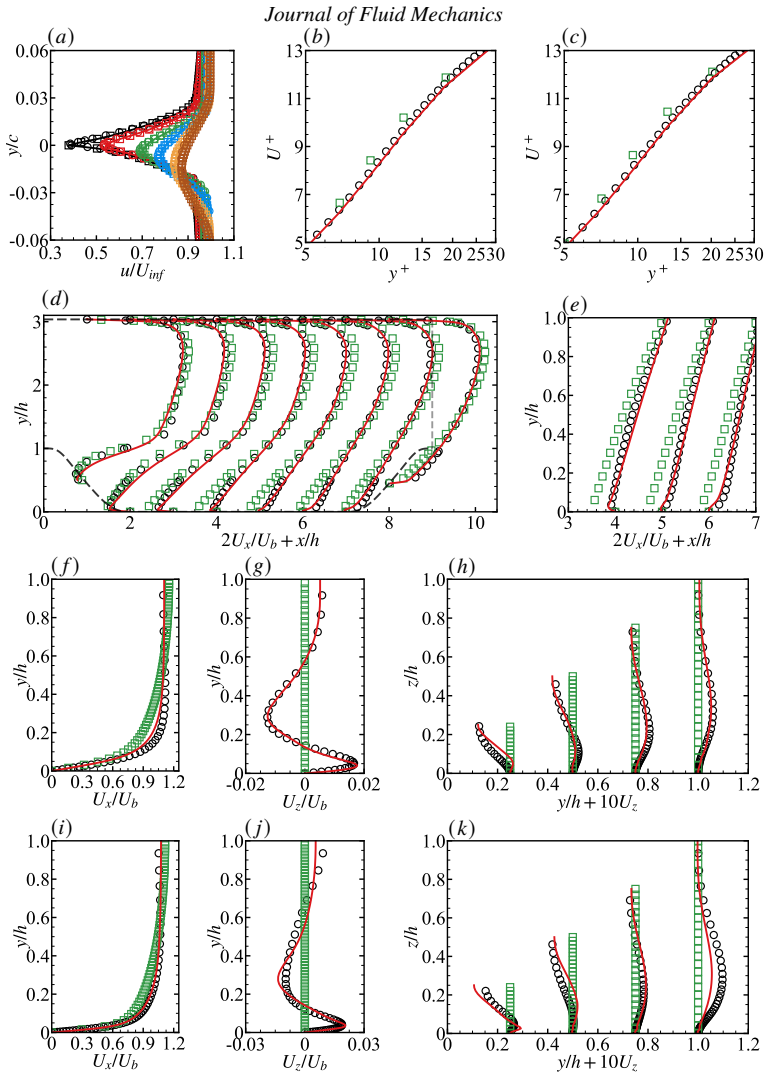
- [§4.2–4.3] The central accuracy claim is supported only by visual profile comparisons in Figs 7 and 8; no quantitative error metric, uncertainty estimate, or convergence data is reported. This makes it impossible to judge the magnitude of the PMoE improvement over the SA baseline or to compare cases. Please add error norms (e.g., L2 relative errors in mean velocity and secondary-flow components) for trained and unseen cases.
- [§2.2.2, Eqs. (2.8)–(2.9)] The information-bottleneck (IB) objective is presented as the training objective of the autoencoder, but the actual loss (Eq. 2.5) is reconstruction MSE and Eq. (2.8) is never optimized. The statement that a minimal feature subset S satisfying Eq. (2.9) follows from the IB Lagrangian is unsupported. This is a methodological overreach that should be removed or replaced by a derivation showing how reconstruction training implements IB.
- [§2.2.2 and §4] The acceptance threshold T_accept=90% and the sampling threshold epsilon=0.05 are fixed and calibrated on the four regimes considered; no sensitivity analysis is given, and the paper admits T_accept would need tuning in future applications. The claim that the router 'detects when a flow is not represented' is therefore demonstrated only for well-separated regimes with the chosen features. A concrete test on a held-out flow family (e.g., a curved duct or airfoil separation) and a sensitivity study of T_accept would be needed to support the novelty-detection claim.
minor comments (5)
- [§3.2, §3.4, §4.2] Typos: 'weel' should be 'well' (§3.2); 'shwon' should be 'shown' (§3.4); 'at at' duplicated (§4.2).
- [Figure 5] Caption contains 'DNSbaselineexpert' with missing separators; format consistently throughout.
- [§2.2.1, Appendix A] The PFI analysis is presented as motivation, but the router uses the full seven features. Clarify whether PFI is an interpretability diagnostic only or actually informs feature selection.
- [§2.2.2] The term 'confidence' for p_k is potentially misleading, as p_k is a recognition rate based on reconstruction-error thresholding, not a calibrated probability. Consider renaming it 'recognition rate' or similar.
- [General] No data or code availability statement is provided. Please include access details for training data and expert implementations, as reproducibility is important for a data-driven modelling paper.
Circularity Check
Router self-recognition confidence is definitional and internally inconsistent; out-of-sample expert validation is independent.
-
self definitional
[§2.2.2 (Eqs. 2.5–2.6), Table 3, §3.3]
"After the training of the kth router component C_k is converged, we set the 99.9th percentile of the reconstruction error of the training data as the corresponding threshold T_k ... p_k = N_k/N, where N_k = Σ_j I(L_j < T_k) ... Table 3: 'Confidence of new router component 99.9% 99.5% 93.5% 97.0%' ... 'the identification confidence for separated flows rises to 93.5%'."
T_k is defined as the 99.9th percentile of the training-data reconstruction errors, and p_k is defined as the fraction of points with error below T_k. Therefore, on the same training data used to set T_k, p_k is approximately 99.9% by construction. The paper presents the 'Confidence of new router component' (Table 3) and statements such as 'the identification confidence for separated flows rises to 93.5%' as evidence that the newly added router component recognizes the new regime. If these values are computed on that component's own training data, high confidence is guaranteed rather than demonstrated; if computed on other data, the paper does not specify this, and the reported values (93.5%, 97.0%; Table 5 lists 91.5% for PH1p0 and 97.0% for SD5693, both training cases) contradict the sta
full rationale
The core generalization evidence is independent: unseen cases C8000, PH0p8, PH1p2, PH1p5, and SD3500 are not used to train the experts or router components, and the expert corrections (SR damping function, FIML production correction, QCR coefficient field) are fitted to different training cases and then assessed on those held-out flows. The old-router confidences assigned to genuinely new regimes (0.0% for channel after wake, 58.4% for periodic hill, 56.7% for square duct) are also empirical, not forced by construction. There is no load-bearing self-citation chain or imported uniqueness theorem; the method builds on standard external references. The circularity is confined to the router's self-recognition demonstration: because each T_k is the 99.9th percentile of that component's training errors, p_k on the same training data is ~99.9% by definition, so reporting such confidences as evidence of correct routing is not independent. Moreover, the reported values are inconsistent with the stated threshold protocol, further weakening this particular validation. Since the out-of-sample accuracy and forgetting-prevention results remain genuinely self-contained, the score is moderate rather than high.
Assumptions & free parameters
free parameters (8)
- Acceptance threshold T_accept =
90%
- Sampling threshold epsilon =
0.05
- Autoencoder bottleneck dimension =
4
- Reconstruction threshold percentile =
99.9th percentile per component
- Damping-function correction coefficients =
0.985, 1.3, 31.1
- Production-correction field beta(x) =
FI-NN weights trained on PH1p0
- QCR coefficient field C_cr1(x) =
FI-NN weights trained on SD2500/SD5693
- Number of sampled points N =
10000
assumptions (6)
- domain assumption SA baseline model provides a meaningful starting closure for all four regimes
- ad hoc to paper Autoencoder reconstruction error on the seven selected features is a valid similarity metric for flow regimes
- ad hoc to paper Winner-takes-all top-1 routing with T_accept=90% correctly separates known from novel regimes
- domain assumption The seven features in Table 1 are sufficient to distinguish the regimes tested
- ad hoc to paper Information bottleneck argument implies a minimal informative feature subset and that the autoencoder latent representation isolates flow-specific features
- domain assumption Corrections learned in one flow of a family transfer to other geometries/Reynolds numbers in the same family
Cite this review
Pith. "Pith review of Progressive Mixture-of-Experts with autoencoder routing for continual RANS turbulence modelling." pith.science (2026). https://pith.science/paper/DHQ7KBZU
@misc{pith2026260109305,
  author       = {Pith},
  title        = {Pith review of: Progressive Mixture-of-Experts with autoencoder routing for continual RANS turbulence modelling},
  year         = {2026},
  howpublished = {\url{https://pith.science/paper/DHQ7KBZU}},
  note         = {Machine review of arXiv:2601.09305}
}
read the original abstract
Developing Reynolds-averaged Navier-Stokes (RANS) turbulence models that remain accurate across diverse flow regimes is a long-standing challenge. In this work, we propose a novel framework, termed the progressive mixture-of-experts (PMoE), designed to enable continual learning for RANS turbulence modelling. The framework employs a modular autoencoder-based router to associate each flow scenario with a specialised turbulence model, referred to as an expert. When a new flow regime cannot be adequately represented by the existing router and expert set, a new expert together with its routing component can be introduced at low cost, without modifying or degrading previously trained ones, thereby naturally avoiding catastrophic forgetting. The framework is applied to a range of flows with distinct physical characteristics, including airfoil wake, channel, periodic hill, and square duct flows. The resulting PMoE model effectively integrates multiple experts and achieves improved predictive accuracy across both seen and unseen test cases that differ in operating conditions or configurations. Owing to sparse activation, model expansion does not incur additional computational cost during inference. The proposed framework therefore provides a scalable pathway towards lifelong-learning turbulence models for industrial computational fluid dynamics.
Figures


Figures from the paper (7 more)




Reference graph
Works this paper leans on
-
[1]
& Abkar, M.2023 Progressive augmentation of turbulence models for flow separation by multi-case computational fluid dynamics driven surrogate optimization.Phys
Amarloo, A., Rinc´on, M.J., Reclari, M. & Abkar, M.2023 Progressive augmentation of turbulence models for flow separation by multi-case computational fluid dynamics driven surrogate optimization.Phys. Fluids 35(12), 125154. Arranz, G., Ling, Y., Costa, S., Goc, K. & Lozano-Dur ´an, A.2024 Building-block-flow computational model for large-eddy simulation o...
2023
-
[3]
Mandler, H
Mahalanobis, P.C.1936 On the generalised distance in statistics.Proceedings of the National Institute of Science of India2, 49–55. Mandler, H. & Weigand, B.2023 Feature importance in neural networks as a means of interpretation for data-driven turbulence models.Comp. Fluids265, 105993. Menter, F.R.1994 Two-equation eddy-viscosity turbulence models for eng...
1936
-
[127]
& Yang, X.I.A.2023 Data-enabled recalibration of the Spalart–Allmaras model.AIAA J
Bin, Y., Huang, G. & Yang, X.I.A.2023 Data-enabled recalibration of the Spalart–Allmaras model.AIAA J. 61(11), 4852–4863. Breiman, L.2001 Random forests.Machine learning45(1), 5–32. Brunton, S.L., Noack, B.R. & Koumoutsakos, P.2020 Machine learning for fluid mechanics.Ann. Rev. Fluid Mech.52, 477–508. Bush, R.H., Chyczewski, T.S., Duraisamy, K., Eisfeld, ...
2023
-
[201]
& Coleman, G.N.2022 NASA symposium on turbulence modeling: Roadblocks, and the potential for machine learning
Rumsey, C.L. & Coleman, G.N.2022 NASA symposium on turbulence modeling: Roadblocks, and the potential for machine learning. Technical report. Langley Research Center, Hampton, V A, USA. Sandberg, R.D. & Zhao, Y.2022 Machine-learning for turbulence and heat-flux model development: A review of challenges associated with distinct physical phenomena and progr...
2022
-
[317]
& Gloerfelt, X.2025 Space-dependent aggregation of stochastic data-driven turbulence models.J
Cherroud, S., Merle, X., Cinnella, P. & Gloerfelt, X.2025 Space-dependent aggregation of stochastic data-driven turbulence models.J. Comp. Phys.527, 113793. Dai, D., Deng, C., Zhao, C., Xu, R.X., Gao, H., Chen, D., Li, J., Zeng, W., Yu, X., Wu, Y., Xie, Z., Li, Y.k., Huang, P., Luo, F., Ruan, C., Sui, Z. & Liang, W.2024 DeepSeekMoE: Towards ultimate exper...
2025
-
[439]
& Bialek, W.2000 The information bottleneck method.arXiv preprint physics/0004057
Tishby, N., Pereira, F.C. & Bialek, W.2000 The information bottleneck method.arXiv preprint physics/0004057. Vinuesa, R., Schlatter, P. & Nagib, H.M.2018 Secondary flow in turbulent ducts with increasing aspect ratio.Phys. Rev. Fluids3(5), 054606. Wang, J., Wu, J. & Xiao, H.2017 Physics-informed machine learning approach for reconstructing reynolds stress...
arXiv 2000
-
[1284]
& Sandberg, R.D.2023 Toward more general turbulence models via multicase computational-fluid-dynamics-driven training.AIAA J.61(5), 2100–2115
Fang, Y., Zhao, Y., Waschkowski, F., Ooi, A.S.H. & Sandberg, R.D.2023 Toward more general turbulence models via multicase computational-fluid-dynamics-driven training.AIAA J.61(5), 2100–2115. Fedus, W., Zoph, B. & Shazeer, N.2022 Switch transformers: scaling to trillion parameter models with simple and efficient sparsity.J. Mach. Learn. Res.23(120), 1–39....
2023
Reviewed August 3, 2026 · model on record in the stance chip above.
Discussion (0). Continue with ORCID to comment.