REVIEW 3 major objections 5 minor 1 cited by
This paper claims that in two-stage axion monodromy inflation, the end of the heavy-axion stage can trigger exponential dark U(1) gauge-field production, sourcing a narrow gravitational-wave spike today at 10–500 kHz with amplitude within r
Reviewed by Pith at T0; open to challenge. T0 means a machine referee read the full paper against a public rubric. the ladder, T0–T4 →
T0 review · deepseek-v4-flash
2026-08-03 10:28 UTC pith:KFWH6QZT
load-bearing objection Solid, clearly-written phenomenology: the new piece is placing the double-monodromy break at N_CMB=50-52, shifting the known axion-U(1)-to-GW spike into 10 kHz-300 kHz with concrete LSD/ET sensitivity estimates -- but the peak amplitude sits in the backreaction grey zone the paper flags without resolving. the 3 major comments →
Very-High-Frequency Gravitational Waves from Multi-Monodromy Inflation
The pith
A machine-rendered reading of the paper's core claim, the machinery that carries it, and where it could break.
Core claim
The central claim is that in a two-axion monodromy model where the heavier axion couples to a dark U(1) gauge field, the interruption near the end of the first stage acts as a source of strongly chiral, sharply peaked gravitational waves. The peak frequency is set by the number of efolds between the break and the end of inflation: placing the break at ΔN_e ≈ 50–52 puts the signal in the 10–300 kHz band, with a strain that approaches the sensitivity of proposed levitated-sensor detectors; placing it earlier shifts the peak to lower frequencies accessible to other observatories. The amplitude is controlled by the gauge-production parameter ξ = φ̇/(2Hf_φ); for ξ ≳ 3 the gauge fields grow as e^{
What carries the argument
The load-bearing mechanism is the tachyonic instability of one helicity of a dark U(1) gauge field coupled to the rolling axion through the term (φ/4f) F F̃. The efficiency parameter ξ = φ̇/(2Hf_φ) determines the exponent: for ξ ≳ 3, the gauge-field occupation grows like e^{4πξ}, and this chiral gauge radiation converts into gravitational waves with a spectrum peaked at a frequency determined by the Hubble scale at the break and by how many efolds before the end of inflation the break occurs. The two-stage potential V = M_1^4[(1+φ_1^2/μ_1^2)^{p_1/2}−1] + M_2^4[(1+φ_2^2/μ_2^2)^{p_2/2}−1] with M_1 > M_2 produces the 'rollercoaster' trajectory, and the first stage's duration ΔN_e sets the peak
Load-bearing premise
The entire signal rests on the assumption, acknowledged after Eq. (6) and in footnote 2, that the heavy axion's decay constant and dark U(1) coupling make ξ ≈ φ̇/(2Hf_φ) ≳ 3 at the end of its stage; the paper scans f_φ = 0.05–0.15 M_Pl but does not derive from the UV construction that such a sub-Planckian constant, strong coupling, and small Stueckelberg mass all hold. If ξ < 3, the exponential enhancement disappears.
What would settle it
A backreaction-inclusive lattice simulation of the axion–dark-U(1) system at ξ ≈ 3–5 would settle whether the exponential gauge-field growth survives with the assumed efficiency; if the peak Ω_GW h² is quenched below ~10^-8 at 10–300 kHz, the detection claim fails. Alternatively, a null search at a strain sensitivity of ~10^-24 Hz^-1/2 over 10^8 s in the 10–300 kHz band would exclude the optimistic parameter envelope.
If this is right
- If the model is correct, the frequency of the gravitational-wave peak is a direct measure of when the first inflationary stage ended: ΔN_e ≈ 50–52 puts the signal in the 10–300 kHz band, while earlier breaks move it down toward satellite-based interferometer frequencies.
- The narrow width of the peak (Δf/f ≈ 0.1) means the total gravitational-wave energy stays under the BBN/ΔN_eff bound even when the peak amplitude is orders of magnitude above the scale-invariant limit.
- The predicted strain can approach the sensitivity of proposed terrestrial and levitated-sensor detectors with integration times near 10^8 s, making the scenario testable in the near term.
- A detection would simultaneously establish multi-stage inflation and the existence of a dark U(1) sector coupled to the inflaton, bypassing the cosmic no-hair theorem that usually erases such transient dynamics.
- The same mechanism with different break times yields a continuous family of narrow gravitational-wave peaks from nHz to MHz, linking CMB-era observatories to high-frequency detectors.
Where Pith is reading between the lines
- Beyond the paper: the predicted background is chiral, so cross-correlating two nearby detectors should reveal a parity asymmetry; measuring it would distinguish this axionic signal from unpolarized astrophysical backgrounds.
- Beyond the paper: a null result at 10–300 kHz at the quoted strain sensitivity would directly constrain the combination of the heavy axion's decay constant and its dark U(1) coupling, effectively bounding ξ at the exit—an inverse test of the monodromy parameter space.
- Beyond the paper: the paper's frequency–efold relation could be inverted to turn a measured peak frequency into a measurement of the duration of the first inflationary stage, effectively using gravitational-wave detectors as a clock for the internal structure of inflation.
- Beyond the paper: the backreaction uncertainty flagged in the paper suggests that a full lattice simulation of gauge-field production at ξ ≈ 3–5 would sharpen both the peak amplitude and width, determining whether the grey uncertainty region in the figures is real or optimistic.
Editorial analysis
A structured set of objections, weighed in public.
Referee Report
Summary. This paper proposes that in two-stage axion monodromy inflation, the end of the first stage can source a sharply peaked gravitational-wave background through axion coupling to a dark U(1). By choosing the duration of the first stage to be 50–52 efolds (N_CMB=50–52), the peak frequency falls in the 10–300 kHz band, and the amplitude, estimated from Eq. (6), can approach the sensitivity of Einstein Telescope, Cosmic Explorer, and proposed levitated-sensor detectors. The paper argues that the narrow peak evades BBN/ΔN_eff bounds even when its amplitude exceeds broad-band limits. The detector sensitivity section gives a concrete projection for a 10 km levitated sensor with assumed finesse and laser parameters.
Significance. The mechanism is physically plausible and the paper makes a concrete connection between multi-stage inflation and high-frequency gravitational-wave observatories. It uses an established gauge-production formula and provides a first estimate of the reach of a 10 km levitated-sensor detector. If a full treatment confirmed the peak, this would be a striking, falsifiable signature. The paper's main value is as a phenomenological target-setting study. However, the central amplitude estimate is obtained in a regime where the production formula is not reliable, and the parameters that set the frequency and amplitude are scanned rather than derived. The significance is therefore conditional on addressing these points.
major comments (3)
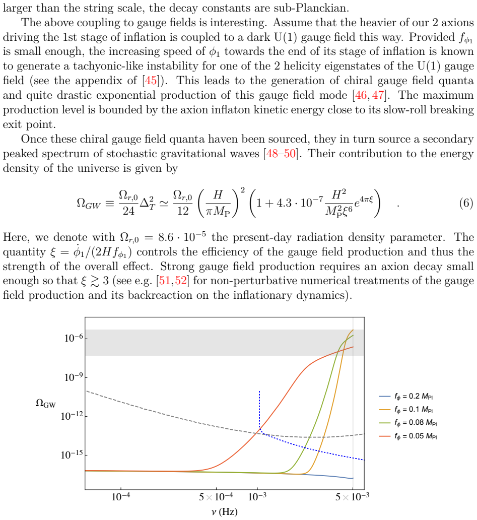
- [§2, Eq. (6); §3, Fig. 4] The central amplitude estimate is obtained from the perturbative formula (6), which contains ξ^6 e^{4πξ}. For the scanned values f_φ1=0.05–0.15 M_Pl and the parameters in Figs. 3–6 (p=0.2, μ1=M_P, M_1^4=2×10^-9 M_P^4), slow-roll at the exit gives ξ ≈ p M_P/(2 f_φ1 φ_end) with φ_end≈p M_P/√2, i.e. ξ≈5–15. The same literature cited for ξ≳3 (refs. [51,52]) shows that backreaction of the produced gauge modes becomes important for ξ≳3–4. The paper labels this a 'grey area' in Fig. 4 but still draws the detection curves in Fig. 6 from the un-backreacted expression. Because the amplitude is exponential in ξ, a backreaction-induced cap on ξ can lower the peak by orders of magnitude and move it below the LSD sensitivity. This needs a quantitative treatment or a restriction to a regime where Eq. (6) is valid.
- [§3, Fig. 5] The predicted peak shape and width are not computed. The text states Δf_p ≃ f_p/10 and adds 'this is a rough estimate' without a derivation, and Fig. 5 is labelled a 'rising edge' only; the full spectrum is not shown. The detector SNR estimate (Eq. 16) integrates over a window Δf ≲ Δf_p, and the BBN check (Eq. 14) depends on the total integrated power. An asserted width and an unshown peak shape are therefore load-bearing for the detectability claim. Please provide the actual ΩGW(f) from the field evolution, or at least a conservative envelope and a clear statement that the width is an assumption.
- [§2, Eq. (7); §3, Figs. 3–6] The two outputs that define the signal are set by hand. Eq. (7) is used to choose N_CMB=50–52 so that the peak falls in the kHz band, and f_φ1 is scanned over 0.05–0.15 M_Pl to set the amplitude. The text says these can be arranged by initial field values, but no model prior or naturalness argument is given, nor is it demonstrated that a sub-Planckian f_φ1 with the required coupling and no Stueckelberg mass is realizable in the monodromy construction. This turns the abstract's 'are in the frequency range ... accessible' into a conditional existence statement. Please state the parameter ranges as a scan and discuss the plausibility of the required values.
minor comments (5)
- [§3] The statement 'Δf_p ≃ 1/10 f_p ... should be correct by order of magnitude' should be presented as an assumption, not a result, unless a derivation or simulation is provided.
- [§4, Tables 1–2] The table captions refer to 'Tables 4 and 4'; these should be 'Table 1 and Table 2'. The figure labels also contain Mathematica 'Out[]' artifacts that should be removed.
- [§4, Eq. (15)] The definitions of h_limit and h_min are not fully consistent in the text: Eq. (15) defines h_limit, while the tables quote h_min = h_limit/√b. Please clarify the relationship explicitly.
- [§2, Eq. (7)] The variable N in Eq. (7) is not defined precisely. It would help to state that N is the number of e-folds before the end of inflation at which the mode exits the horizon.
- [§2] The text mentions that 'the ∼7 observable efolds of the CMB will arise only from the part of inflation driven by the heavier axion', but the later choice N_CMB=50–52 is not connected to this statement. Clarify the role of the second stage and the number of e-folds after the break.
Circularity Check
No significant circularity: the GW spectrum uses external gauge-production formulas; scanned parameters (N_CMB, f_phi1) are model inputs, not fitted outputs.
full rationale
The paper's central signal is assembled from external, independently reproducible ingredients. The GW abundance formula, Eq. (6), is taken from Refs. [48-50] (Barnaby-Pajer-Peloso, Cook-Sorbo, Domcke et al.), not from the paper's own ansatz, and no parameter is fitted to data. The peak frequency is set through Eq. (7), the standard relation between efold number and comoving frequency, with N_CMB chosen via initial field values; the paper transparently scans N_CMB = 50-52 and f_phi1 = 0.05-0.15 M_Pl. Such parameter scans are model-space exploration, not 'prediction of a fitted quantity': the paper does not claim these values are uniquely forced by data. The multi-stage ('rollercoaster') setup is adopted from self-cited work [10,22,23], but it is a model premise rather than a theorem derived from the target result; the gauge-production and detector-sensitivity inputs are independent of those citations. The 'unique 4D EFT' description from [6,39] is a framework preference, not a load-bearing uniqueness proof that forbids alternatives. The acknowledged grey area from backreaction (Fig. 4) and the requirement ξ≳3 are robustness/regime-of-validity concerns about Eq. (6), not a demonstration that the output equals an input by construction. Thus there is no specific circular reduction that can be quoted.
Axiom & Free-Parameter Ledger
free parameters (6)
- f_phi1 (heavy-axion decay constant) =
0.05–0.15 M_Pl (scanned; 0.1 M_Pl central in Fig. 6)
- N_CMB / ΔNe (break time) =
35 (Fig.3), 50, 51, 52 (Figs.4–6)
- M_1^4 (normalization of heavy-axion potential) =
2×10^-9 M_P^4 in Fig.3
- μ1, p1 (flattening parameters) =
μ1=M_P, p1=0.2 (Fig.3); p1=2/5 (Fig.2)
- M_2/M_1 (mass hierarchy) =
0.1 in Fig.2
- Δf/f (peak width) =
~0.1, up to 0.2
axioms (6)
- domain assumption Axion monodromy flattening potential V(ϕ)=M^4[(1+ϕ^2/μ^2)^{p/2}-1] with 0.1≲p<1, Eq.(3).
- ad hoc to paper Two-stage 'rollercoaster' inflation with mass hierarchy, Eq.(4), and initial displacements arranged so the first stage lasts ΔNe efolds.
- domain assumption Coupling of the heavy axion to a dark U(1) gauge field, Eq.(5), with f_phi sub-Planckian and no Stueckelberg mass, and efficiency ξ≳3.
- domain assumption Gauge-field production and GW abundance formula ΩGW = Ωr,0/24 Δ_T^2 ≃ ... Eq.(6) from refs [48-50].
- domain assumption The signal is stationary, Gaussian, isotropic and unpolarized, Eqs.(8)-(9).
- ad hoc to paper The 10 km levitated sensor can achieve the assumed finesse/noise with an additional focusing lens, Tables 1–2.
read the original abstract
We show that in multi-stage axion monodromy inflation an interruption near the end of the penultimate stage can lead to a spike in the gravitational wave background. These gravitational waves are in the frequency range and with an amplitude accessible to proposed terrestrial detectors such as the Einstein Telescope, Cosmic Explorer, and future Levitated Sensor Detector experiments.
Figures




Forward citations
Cited by 1 Pith paper
-
The End of the First Act: Spectral Running, Interacting Dark Radiation, and the Hubble Tension in Light of ACT DR6 Data
Including spectral running α_s, β_s and self-interacting dark radiation relaxes the ACT DR6 bound on ΔN_eff to <0.58 and lowers the Hubble tension to 2.2σ with three extra parameters.
Reference graph
Works this paper leans on
-
[1]
The Inflationary Universe: A Possible Solution to the Horizon and Flatness Problems,
A. H. Guth, “The Inflationary Universe: A Possible Solution to the Horizon and Flatness Problems,” Adv. Ser. Astrophys. Cosmol. 3 (1987) 139–148
1987
-
[2]
A New Inflationary Universe Scenario: A Possible Solution of the Horizon, Flatness, Homogeneity, Isotropy and Primordial Monopole Problems,
A. D. Linde, “A New Inflationary Universe Scenario: A Possible Solution of the Horizon, Flatness, Homogeneity, Isotropy and Primordial Monopole Problems,” Adv. Ser. Astrophys. Cosmol. 3 (1987) 149–153 . 15
1987
-
[3]
Cosmology for Grand Unified Theories with Radiatively Induced Symmetry Breaking,
A. Albrecht and P. J. Steinhardt, “Cosmology for Grand Unified Theories with Radiatively Induced Symmetry Breaking,” Adv. Ser. Astrophys. Cosmol. 3 (1987) 158–161
1987
-
[4]
D. H. Lyth, “What would we learn by detecting a gravitational wave signal in the cosmic microwave background anisotropy?,” Phys. Rev. Lett. 78 (1997) 1861–1863 , arXiv:hep-ph/9606387
Pith/arXiv arXiv 1997
-
[5]
G. Efstathiou and K. J. Mack, “The Lyth Bound Revisited,” JCAP 0505 (2005) 008 , arXiv:astro-ph/0503360
Pith/arXiv arXiv 2005
-
[6]
An Ignoble Approach to Large Field Inflation,
N. Kaloper, A. Lawrence, and L. Sorbo, “An Ignoble Approach to Large Field Inflation,” JCAP 1103 (2011) 023 , arXiv:1101.0026 [hep-th]
Pith/arXiv arXiv 2011
-
[7]
TASI lectures on cosmological observables and string theory,
E. Silverstein, “TASI lectures on cosmological observables and string theory,” in Theoretical Advanced Study Institute in Elementary Particle Physics: New Frontiers in Fields and Strings , pp. 545–606. 2017. arXiv:1606.03640 [hep-th]
Pith/arXiv arXiv 2017
-
[8]
Asymptotic behavior of homogeneous cosmological models in the presence of a positive cosmological constant,
R. M. Wald, “Asymptotic behavior of homogeneous cosmological models in the presence of a positive cosmological constant,” Phys. Rev. D 28 (1983) 2118–2120
1983
-
[9]
Quantum Cosmic No-Hair Theorem and Inflation,
N. Kaloper and J. Scargill, “Quantum Cosmic No-Hair Theorem and Inflation,” Phys. Rev. D 99 no. 10, (2019) 103514 , arXiv:1802.09554 [hep-th]
Pith/arXiv arXiv 2019
-
[10]
G. D’Amico and N. Kaloper, “Rollercoaster cosmology,” JCAP 08 (2021) 058 , arXiv:2011.09489 [hep-th]
Pith/arXiv arXiv 2021
-
[11]
Inflationary Universe Generated by the Combined Action of a Scalar Field and Gravitational Vacuum Polarization,
L. A. Kofman, A. D. Linde, and A. A. Starobinsky, “Inflationary Universe Generated by the Combined Action of a Scalar Field and Gravitational Vacuum Polarization,” Phys. Lett. B 157 (1985) 361–367
1985
-
[12]
Multicomponent de Sitter (Inflationary) Stages and the Generation of Perturbations,
A. A. Starobinsky, “Multicomponent de Sitter (Inflationary) Stages and the Generation of Perturbations,” JETP Lett. 42 (1985) 152–155
1985
-
[13]
Double Inflation,
J. Silk and M. S. Turner, “Double Inflation,” Phys. Rev. D 35 (1987) 419
1987
-
[14]
What kinds of perturbation spectra can be produced by inflation?,
V. F. Mukhanov and M. I. Zelnikov, “What kinds of perturbation spectra can be produced by inflation?,” Phys. Lett. B 263 (1991) 169–175
1991
-
[15]
Spectra of perturbations produced by double inflation with an intermediate matter dominated stage,
D. Polarski and A. A. Starobinsky, “Spectra of perturbations produced by double inflation with an intermediate matter dominated stage,” Nucl. Phys. B 385 (1992) 623–650
1992
-
[16]
Primordial Tensor Perturbation in Double Inflationary Scenario with a Break,
S. Pi, M. Sasaki, and Y.-l. Zhang, “Primordial Tensor Perturbation in Double Inflationary Scenario with a Break,” JCAP 06 (2019) 049 , arXiv:1904.06304 [gr-qc]
Pith/arXiv arXiv 2019
-
[17]
T. Damour and V. F. Mukhanov, “Inflation without slow roll,” Phys. Rev. Lett. 80 (1998) 3440–3443 , arXiv:gr-qc/9712061. 16
Pith/arXiv arXiv 1998
-
[18]
J. A. Adams, G. G. Ross, and S. Sarkar, “Multiple inflation,” Nucl. Phys. B503 (1997) 405–425 , arXiv:hep-ph/9704286
Pith/arXiv arXiv 1997
-
[19]
Multiple inflation, cosmic string networks and the string landscape,
C. P. Burgess, R. Easther, A. Mazumdar, D. F. Mota, and T. Multamaki, “Multiple inflation, cosmic string networks and the string landscape,” JHEP 05 (2005) 067 , arXiv:hep-th/0501125
Pith/arXiv arXiv 2005
-
[20]
Just enough inflation: power spectrum modifications at large scales,
M. Cicoli, S. Downes, B. Dutta, F. G. Pedro, and A. Westphal, “Just enough inflation: power spectrum modifications at large scales,” JCAP 12 (2014) 030 , arXiv:1407.1048 [hep-th]
Pith/arXiv arXiv 2014
-
[21]
A. Arvanitaki, S. Dimopoulos, S. Dubovsky, N. Kaloper, and J. March-Russell, “String Axiverse,” Phys. Rev. D81 (2010) 123530 , arXiv:0905.4720 [hep-th]
Pith/arXiv arXiv 2010
-
[22]
Double Monodromy Inflation: A Gravity Waves Factory for CMB-S4, LiteBIRD and LISA,
G. D’Amico, N. Kaloper, and A. Westphal, “Double Monodromy Inflation: A Gravity Waves Factory for CMB-S4, LiteBIRD and LISA,” Phys. Rev. D 104 no. 8, (2021) L081302, arXiv:2101.05861 [hep-th]
Pith/arXiv arXiv 2021
-
[23]
General double monodromy inflation,
G. D’Amico, N. Kaloper, and A. Westphal, “General double monodromy inflation,” Phys. Rev. D 105 no. 10, (2022) 103527 , arXiv:2112.13861 [hep-th]
Pith/arXiv arXiv 2022
-
[24]
Ultrahigh frequency primordial gravitational waves beyond the kHz: The case of cosmic strings,
G. Servant and P. Simakachorn, “Ultrahigh frequency primordial gravitational waves beyond the kHz: The case of cosmic strings,” Phys. Rev. D 109 no. 10, (2024) 103538 , arXiv:2312.09281 [hep-ph]
Pith/arXiv arXiv 2024
-
[25]
Exploring the Sensitivity of Next Generation Gravitational Wave Detectors,
LIGO Scientific Collaboration, B. P. Abbott et al. , “Exploring the Sensitivity of Next Generation Gravitational Wave Detectors,” Class. Quant. Grav. 34 no. 4, (2017) 044001, arXiv:1607.08697 [astro-ph.IM]
Pith/arXiv arXiv 2017
-
[26]
Sensitivity Studies for Third-Generation Gravitational Wave Observatories,
S. Hild et al. , “Sensitivity Studies for Third-Generation Gravitational Wave Observatories,” Class. Quant. Grav. 28 (2011) 094013 , arXiv:1012.0908 [gr-qc]
Pith/arXiv arXiv 2011
-
[27]
Search for the isotropic stochastic background using data from Advanced LIGO’s second observing run,
LIGO Scientific, Virgo Collaboration, B. P. Abbott et al. , “Search for the isotropic stochastic background using data from Advanced LIGO’s second observing run,” Phys. Rev. D 100 no. 6, (2019) 061101 , arXiv:1903.02886 [gr-qc]
Pith/arXiv arXiv 2019
-
[28]
The Einstein Telescope: A third-generation gravitational wave observatory,
M. Punturo et al. , “The Einstein Telescope: A third-generation gravitational wave observatory,” Class. Quant. Grav. 27 (2010) 194002
2010
-
[29]
Characterization of the LIGO detectors during their sixth science run,
LIGO Scientific, VIRGO Collaboration, J. Aasi et al. , “Characterization of the LIGO detectors during their sixth science run,” Class. Quant. Grav. 32 no. 11, (2015) 115012, arXiv:1410.7764 [gr-qc]
Pith/arXiv arXiv 2015
-
[30]
Cosmology with the Laser Interferometer Space Antenna,
LISA Cosmology Working Group Collaboration, P. Auclair et al. , “Cosmology with the Laser Interferometer Space Antenna,” Living Rev. Rel. 26 no. 1, (2023) 5 , arXiv:2204.05434 [astro-ph.CO] . 17
Pith/arXiv arXiv 2023
-
[31]
Challenges and opportunities of gravitational-wave searches at MHz to GHz frequencies,
N. Aggarwal et al. , “Challenges and opportunities of gravitational-wave searches at MHz to GHz frequencies,” Living Rev. Rel. 24 no. 1, (2021) 4 , arXiv:2011.12414 [gr-qc]
Pith/arXiv arXiv 2021
-
[32]
Laser interferometer space antenna,
P. A.-S. et al., “Laser interferometer space antenna,” 2017. https://arxiv.org/abs/1702.00786
Pith/arXiv arXiv 2017
-
[33]
Detector configuration of DECIGO/BBO and identification of cosmological neutron-star binaries,
K. Yagi and N. Seto, “Detector configuration of DECIGO/BBO and identification of cosmological neutron-star binaries,” Phys. Rev. D 83 (2011) 044011 , arXiv:1101.3940 [astro-ph.CO] . [Erratum: Phys.Rev.D 95, 109901 (2017)]
Pith/arXiv arXiv 2011
-
[34]
AEDGE: Atomic Experiment for Dark Matter and Gravity Exploration in Space,
AEDGE Collaboration, Y. A. El-Neaj et al. , “AEDGE: Atomic Experiment for Dark Matter and Gravity Exploration in Space,” EPJ Quant. Technol. 7 (2020) 6 , arXiv:1908.00802 [gr-qc]
Pith/arXiv arXiv 2020
-
[35]
KAGRA, LIGO Scientific, Virgo Collaboration, B. P. Abbott et al. , “Prospects for observing and localizing gravitational-wave transients with Advanced LIGO, Advanced Virgo and KAGRA,” Living Rev. Rel. 19 (2016) 1 , arXiv:1304.0670 [gr-qc]
Pith/arXiv arXiv 2016
-
[36]
Bridging the µHz Gap in the Gravitational-Wave Landscape with Binary Resonances,
D. Blas and A. C. Jenkins, “Bridging the µHz Gap in the Gravitational-Wave Landscape with Binary Resonances,” Phys. Rev. Lett. 128 no. 10, (2022) 101103 , arXiv:2107.04601 [astro-ph.CO]
Pith/arXiv arXiv 2022
-
[37]
Asteroids for µHz gravitational-wave detection,
M. A. Fedderke, P. W. Graham, and S. Rajendran, “Asteroids for µHz gravitational-wave detection,” Phys. Rev. D 105 no. 10, (2022) 103018 , arXiv:2112.11431 [gr-qc]
Pith/arXiv arXiv 2022
-
[38]
Gravity Waves and Linear Inflation from Axion Monodromy,
L. McAllister, E. Silverstein, and A. Westphal, “Gravity Waves and Linear Inflation from Axion Monodromy,” Phys.Rev. D82 (2010) 046003 , arXiv:0808.0706 [hep-th]
Pith/arXiv arXiv 2010
-
[39]
A Natural Framework for Chaotic Inflation,
N. Kaloper and L. Sorbo, “A Natural Framework for Chaotic Inflation,” Phys. Rev. Lett. 102 (2009) 121301 , arXiv:0811.1989 [hep-th]
Pith/arXiv arXiv 2009
-
[40]
Simple exercises to flatten your potential,
X. Dong, B. Horn, E. Silverstein, and A. Westphal, “Simple exercises to flatten your potential,” Phys.Rev. D84 (2011) 026011 , arXiv:1011.4521 [hep-th]
Pith/arXiv arXiv 2011
-
[41]
London equation for monodromy inflation,
N. Kaloper and A. Lawrence, “London equation for monodromy inflation,” Phys. Rev. D 95 no. 6, (2017) 063526 , arXiv:1607.06105 [hep-th]
Pith/arXiv arXiv 2017
-
[42]
Three-form gauging of axion symmetries and gravity,
G. Dvali, “Three-form gauging of axion symmetries and gravity,” arXiv:hep-th/0507215
-
[43]
Monodromy Inflation in the Strong Coupling Regime of the Effective Field Theory,
G. D’Amico, N. Kaloper, and A. Lawrence, “Monodromy Inflation in the Strong Coupling Regime of the Effective Field Theory,” Phys. Rev. Lett. 121 no. 9, (2018) 091301, arXiv:1709.07014 [hep-th] . 18
Pith/arXiv arXiv 2018
-
[44]
M. Dias, J. Frazer, and A. Westphal, “Inflation as an Information Bottleneck - A strategy for identifying universality classes and making robust predictions,” JHEP 05 (2019) 065 , arXiv:1810.05199 [hep-th]
Pith/arXiv arXiv 2019
-
[45]
Physical properties of four-dimensional superstring gravity black hole solutions,
B. A. Campbell, N. Kaloper, R. Madden, and K. A. Olive, “Physical properties of four-dimensional superstring gravity black hole solutions,” Nucl. Phys. B 399 (1993) 137–168, arXiv:hep-th/9301129
Pith/arXiv arXiv 1993
-
[46]
M. M. Anber and L. Sorbo, “N-flationary magnetic fields,” JCAP 0610 (2006) 018, arXiv:astro-ph/0606534
Pith/arXiv arXiv 2006
-
[47]
Naturally inflating on steep potentials through electromagnetic dissipation,
M. M. Anber and L. Sorbo, “Naturally inflating on steep potentials through electromagnetic dissipation,” Phys.Rev. D81 (2010) 043534 , arXiv:0908.4089 [hep-th]
Pith/arXiv arXiv 2010
-
[48]
N. Barnaby, E. Pajer, and M. Peloso, “Gauge Field Production in Axion Inflation: Consequences for Monodromy, non-Gaussianity in the CMB, and Gravitational Waves at Interferometers,” Phys. Rev. D 85 (2012) 023525 , arXiv:1110.3327 [astro-ph.CO]
Pith/arXiv arXiv 2012
-
[49]
J. L. Cook and L. Sorbo, “Particle production during inflation and gravitational waves detectable by ground-based interferometers,” Phys. Rev. D 85 (2012) 023534 , arXiv:1109.0022 [astro-ph.CO] . [Erratum: Phys.Rev.D 86, 069901 (2012)]
Pith/arXiv arXiv 2012
-
[50]
PBH dark matter from axion inflation,
V. Domcke, F. Muia, M. Pieroni, and L. T. Witkowski, “PBH dark matter from axion inflation,” JCAP 07 (2017) 048 , arXiv:1704.03464 [astro-ph.CO]
Pith/arXiv arXiv 2017
-
[51]
G. Dall’Agata, S. González-Martín, A. Papageorgiou, and M. Peloso, “Warm dark energy,” JCAP 08 (2020) 032 , arXiv:1912.09950 [hep-th]
Pith/arXiv arXiv 2020
-
[52]
Resonant backreaction in axion inflation,
V. Domcke, V. Guidetti, Y. Welling, and A. Westphal, “Resonant backreaction in axion inflation,” JCAP 09 (2020) 009 , arXiv:2002.02952 [astro-ph.CO]
Pith/arXiv arXiv 2020
-
[53]
Cosmological Backgrounds of Gravitational Waves,
C. Caprini and D. G. Figueroa, “Cosmological Backgrounds of Gravitational Waves,” Class. Quant. Grav. 35 no. 16, (2018) 163001 , arXiv:1801.04268 [astro-ph.CO]
Pith/arXiv arXiv 2018
-
[54]
The Atacama Cosmology Telescope: DR6 Constraints on Extended Cosmological Models,
ACT Collaboration, E. Calabrese et al. , “The Atacama Cosmology Telescope: DR6 Constraints on Extended Cosmological Models,” arXiv:2503.14454 [astro-ph.CO]
-
[55]
SPT-3G Collaboration, E. Camphuis et al. , “SPT-3G D1: CMB temperature and polarization power spectra and cosmology from 2019 and 2020 observations of the SPT-3G Main field,” arXiv:2506.20707 [astro-ph.CO]
Pith/arXiv arXiv 2019
-
[56]
Advanced ligo,
J. Aasi, B. Abbott, R. Abbott, T. Abbott, M. Abernathy, K. Ackley, C. Adams, T. Adams, P. Addesso, R. Adhikari, et al. , “Advanced ligo,” Classical and quantum gravity 32 no. 7, (2015) 074001. 19
2015
-
[57]
Enhanced sensitivity of the ligo gravitational wave detector by using squeezed states of light,
J. e. a. Aasi, “Enhanced sensitivity of the ligo gravitational wave detector by using squeezed states of light,” Nature Photonics 7 no. 8, (Aug, 2013) 613–619 . https://doi.org/10.1038/nphoton.2013.177
-
[58]
Detecting high-frequency gravitational waves with optically levitated sensors,
A. Arvanitaki and A. A. Geraci, “Detecting high-frequency gravitational waves with optically levitated sensors,” Phys. Rev. Lett. 110 (Feb, 2013) 071105 . https://link.aps.org/doi/10.1103/PhysRevLett.110.071105
-
[59]
Searching for new physics with a levitated-sensor-based gravitational-wave detector,
N. Aggarwal, G. P. Winstone, M. Teo, M. Baryakhtar, S. L. Larson, V. Kalogera, and A. A. Geraci, “Searching for new physics with a levitated-sensor-based gravitational-wave detector,” Phys. Rev. Lett. 128 (Mar, 2022) 111101 . https://link.aps.org/doi/10.1103/PhysRevLett.128.111101
-
[60]
Challenges and opportunities of gravitational wave searches above 10 khz,
N. Aggarwal, O. D. Aguiar, D. Blas, A. Bauswein, G. Cella, S. Clesse, A. M. Cruise, V. Domcke, S. Ellis, D. G. Figueroa, G. Franciolini, C. Garcia-Cely, A. Geraci, M. Goryachev, H. Grote, M. Hindmarsh, A. Ito, J. Kopp, S. M. Lee, K. Martineau, J. McDonald, F. Muia, N. Mukund, D. Ottaway, M. Peloso, K. Peters, F. Quevedo, A. Ricciardone, A. Ringwald, J. St...
arXiv 2025
-
[61]
LSD Collaboration Collaboration, G. Winstone, Z. Wang, S. Klomp, R. G. Felsted, A. Laeuger, C. Gupta, D. Grass, N. Aggarwal, J. Sprague, P. J. Pauzauskie, S. L. Larson, V. Kalogera, and A. A. Geraci, “Optical trapping of high-aspect-ratio nayf hexagonal prisms for khz-mhz gravitational wave detectors,” Phys. Rev. Lett. 129 (Jul, 2022) 053604 . https://lin...
-
[62]
Direct measurement of photon recoil from a levitated nanoparticle,
V. Jain, J. Gieseler, C. Moritz, C. Dellago, R. Quidant, and L. Novotny, “Direct measurement of photon recoil from a levitated nanoparticle,” Phys. Rev. Lett. 116 (Jun, 2016) 243601 . https://link.aps.org/doi/10.1103/PhysRevLett.116.243601
-
[63]
Detecting dark-matter waves with a network of precision-measurement tools,
A. Derevianko, “Detecting dark-matter waves with a network of precision-measurement tools,” Phys. Rev. A 97 (Apr, 2018) 042506 . https://link.aps.org/doi/10.1103/PhysRevA.97.042506. 20
discussion (0)
Sign in with ORCID, Apple, or X to comment. Anyone can read and Pith papers without signing in.