REVIEW 3 major objections 4 minor 77 references
Once the universal eikonal carrier of the graviton pole is supplied, the remaining positive spectrum in six dimensions organizes into a cap-saturated low-impact band near the rotating black-hole scale, a separate high-spin ridge, and an emp
Reviewed by Pith at T0; open to challenge. T0 means a machine referee read the full paper against a public rubric. the ladder, T0–T4 →
T0 review · deepseek-v4-flash
2026-08-02 08:26 UTC pith:MQNUBMAW
load-bearing objection A genuinely new, honestly caveated finite-grid SDR bootstrap; the endpoint residual is a real soft spot but not a disqualifier — send to referees. the 3 major comments →
Bootstrapping black holes at low impact parameter
The pith
A machine-rendered reading of the paper's core claim, the machinery that carries it, and where it could break.
Core claim
On its own terms, the paper claims that after the complete high-spin continuum tail of the universal eikonal carrier is inserted, the residual positive spectrum required by the SDR is highly organized rather than featureless. In the scale-reversed microscope (Planck mass below the EFT scale) the extremal witnesses develop a cap-saturated low-impact band near an order-one rotating black-hole guide, a distinct high-spin ridge, and eventually parallel far-tail tracks, while the broad available region between the band and the eikonal layer remains almost empty. In the hierarchy-correct weak-gravity regime the low-spin saturated band has an edge that barely moves as Newton's constant shrinks, and
What carries the argument
The central object is the stringy dispersion relation (SDR) with auxiliary parameter lambda, a crossing-symmetric representation whose large-energy tail probes fixed-t-like kinematics at momentum transfer roughly lambda, giving a continuous family of sum rules. The paper splits the absorptive partial-wave density into a prescribed eikonal carrier, the elastic density 1-cos(chi) built from the six-dimensional Einstein eikonal phase, and an unknown residual density, then discretizes the residual on a (sigma, J) grid and enforces the sampled lambda constraints as a linear program with the unitarity box 0 <= rho <= 2. The workhorse equation is the carrier-complete sum rule A rho_res - lambda^2 Y
Load-bearing premise
The load-bearing premise is that the finite spectral grids, with up to 1200 sigma-nodes and 120 sampled lambda constraints, together with the prescribed eikonal trust region, faithfully encode the continuum stringy dispersion relation over the scales that decide the structure; since the dense residual reaches about two percent exactly at the lambda-to-0 endpoint layer where the graviton-pole behavior lives, the band, gap, and wedge could in principle be truncation artifacts r
What would settle it
A concrete test is to rerun the carrier-complete problem with steadily finer spectral collocation concentrated near lambda = 0 and near the low-energy onset: if the two-percent dense-residual layer does not shrink and the cap-saturated band, the empty gap, or the wedge changes topology, the central organization is a grid artifact. Alternatively, scan an adjustable string-scale alpha' in the prescribed carrier: if the weak-coupling microscopic edge fails to track sqrt(alpha') while the strict zero-gravity null baseline stays put, the band is set by the threshold and the cap, not by a completion
If this is right
- If the central claim is right, the weak-coupling low-impact band is a property of the capped dispersion-relation problem itself, not evidence for a string-to-black-hole crossover; gravity's visible role is to reorganize the support toward the rotating black-hole scale as the coupling grows.
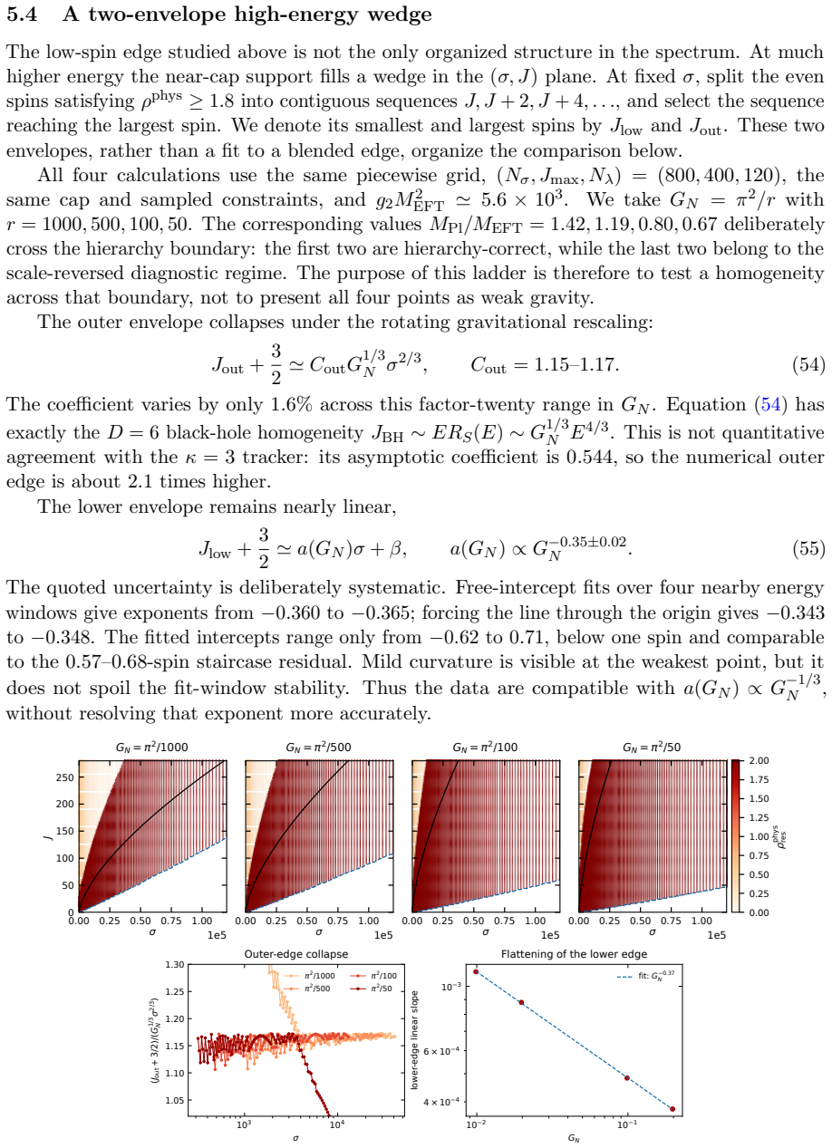
- The high-energy cap-saturated support forms a wedge with an outer envelope J_out + 3/2 ~ C GN^{1/3} sigma^{2/3}, a clean six-dimensional rotating black-hole homogeneity with an order-one coefficient, plus a nearly linear lower envelope whose slope is compatible with GN^{-1/3}, suggesting a Regge-like organization.
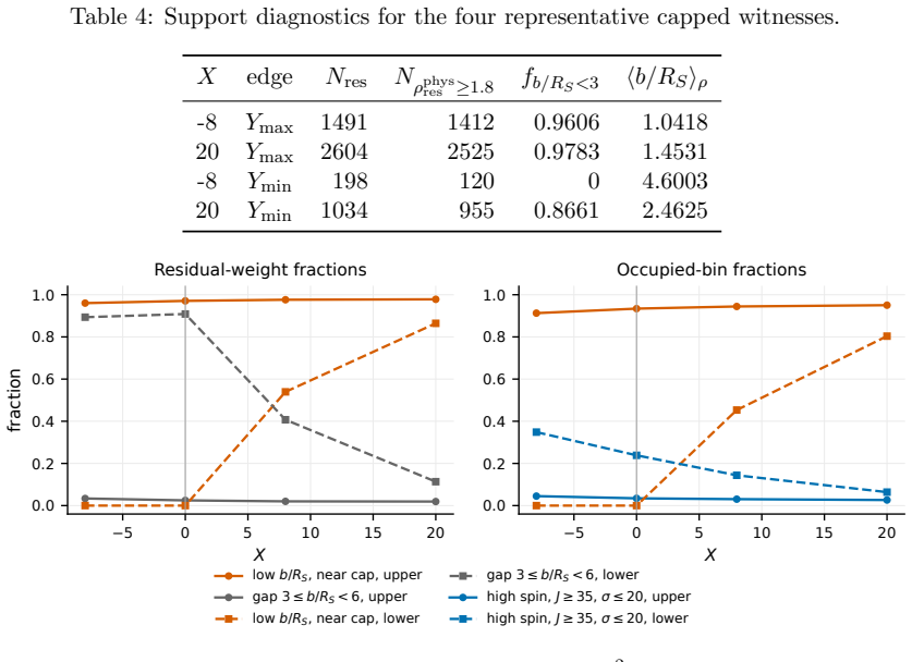
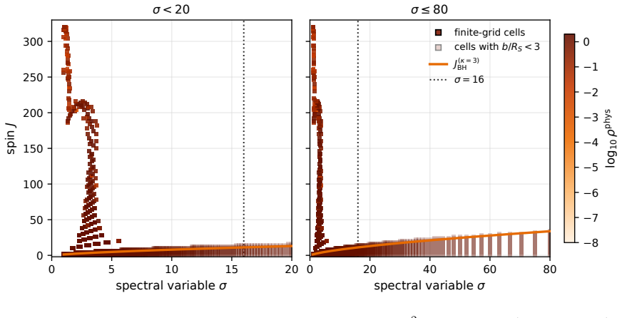
- In the strong-gravity microscope, a cap-saturated low-impact band near the rotating black-hole guide coexists with a separate high-spin ridge, while most available residual bins in between stay unoccupied; reduced costs show that forcing weight into that gap is expensive and that relaxing the cap on the selected band improves the objective.
- The low-impact band is branch-dependent: it is prominent on the upper boundary and the positive-X lower boundary but essentially absent on the negative-X lower boundary, showing the organization is a genuine selection by the extremal problem rather than a generic artifact of cap saturation.
- At the far-energy tail the extremal spectra contain series of nearly parallel, equally spaced tracks at threshold-defined edges, reminiscent of leading and daughter Regge trajectories in dual amplitudes, although they are edges of a continuous density rather than pole locations.
Where Pith is reading between the lines
- Because the strict zero-gravity null already reproduces the weak-coupling band, the decisive next test is whether that band tracks an independent completion scale such as sqrt(alpha'); if it does not, the band is a threshold artifact of the capped SDR and any string/black-hole reading should be dropped.
- The residual dense error peaks around two percent precisely at the lambda-to-0 endpoint layer where the graviton-pole behavior lives; a targeted refinement of spectral collocation near that layer could settle whether the band, gap, and wedge survive in the continuum, a question the paper explicitly leaves open.
- The single-bin kernel-profile sign diagnostic could be exported to other crossing-symmetric bootstrap setups as a cheap pre-solver predictor of where extremal support will land; the paper only gestures at this comparison.
- If the proposed Ericson-type fluctuation width were measured at amplitude level, it would furnish a dynamical, density-independent test of whether the low-impact band behaves like an absorbing black-hole region, which the positive density alone cannot establish.
Editorial analysis
A structured set of objections, weighed in public.
Referee Report
Summary. The paper studies the D=6 stringy dispersion relation (SDR) with a prescribed high-energy, large-impact-parameter eikonal carrier and asks where the remaining positive spectral density is placed. The authors formulate a finite-dimensional linear program over residual partial-wave densities and report several organized structures: a weak-coupling band whose physical impact-parameter edge is nearly fixed as G_N varies and is reproduced by a strict G_N=0 null; a high-energy wedge whose outer envelope scales as G_N^{1/3}\sigma^{2/3} and whose lower envelope is approximately linear with slope compatible with G_N^{-1/3}; and, in a deliberately scale-reversed 'spectral microscope', a cap-saturated low-impact band near a rotating Giddings--Porto black-hole guide, a mostly empty gap, a Regge-like ridge, and far-tail parallel tracks. The paper repeatedly and honestly labels the outputs as finite-grid primal witnesses rather than continuum theorems.
Significance. The question addressed is novel and important: after supplying the universal eikonal carrier, where does the remaining positive spectral weight actually sit? The paper makes several methodical contributions: a carrier-complete source with an analytic high-spin continuum tail, multiple independent source checks (Mathematica and Python), exact agreement between HiGHS dual-simplex and interior-point solves, and ancillary code for reproducibility. The strict G_N=0 null is a clean control that correctly separates non-gravitational baseline effects from genuine strong-gravity organization. If the reported band/gap/wedge structures survive a properly endpoint-resolved calculation, this would be a striking spectral-organization result for gravitational EFT completions. The main caveat is that the load-bearing structures are established only on finite collocation grids, with a percent-level residual concentrated at the small-\lambda endpoint where the carrier cancellation is most singular.
major comments (3)
- [Section 6.4, Table 5, Eq. (60)] The dense off-grid residual \Delta_{\rm dense} saturates at ~0.020 for every refined grid, and the text locates the maximum below the first collocation point \lambda_{\min}=1.07\times10^{-5} (Eq. (32)). This is exactly the layer where the carrier cancellation in Eq. (33) is most singular: F_{\rm eik} carries 1/\lambda and 1/\lambda^2 terms that must cancel against the residual density to reproduce the low-energy EFT target. A 2% mismatch there is not a harmless tail effect. The band/gap/wedge diagnostics (Table 4, Figs. 9-13) are computed from the same finite spectral grid, so they could shift if this endpoint were properly resolved. I would need an endpoint-refined collocation run—e.g., adding \lambda constraints below \lambda_{\min} together with matched spectral endpoint enrichment—before accepting the empty gap and the wedge shape as properties of the full SDR rather than artifacts o
- [Section 6.8] The far-tail 'series of Regge trajectories' is defined by threshold-defined edges at J_{\rm edge}+2k, k=0,...,98. The reported R^2=0.99386 and the exact 2-unit spin separation are therefore built into the construction, not emergent properties of the spectrum. The abstract's claim that 'series of Regge trajectories emerge' overstates what is demonstrated. Please either extract tracks without imposing the 2-unit spacing and show that the spacing emerges independently, or explicitly state that the parallel curves are threshold-defined edges at fixed spacing by definition. As written, this part of the central picture is circular in construction.
- [Section 5.4, Eq. (55)] The lower-envelope exponent is quoted as a(G_N)\propto G_N^{-0.35\pm0.02}, with the systematic range spanning window-dependent fits from -0.360 to -0.348. This is compatible with G_N^{-1/3} but does not establish it. Since the wedge structure is one of the paper's headline results, the abstract and conclusions should state the exponent as 'compatible with -1/3 within fit uncertainty' rather than implying a measured G_N^{-1/3} law. Additional data or a more controlled fitting procedure would be needed to sharpen this point.
minor comments (4)
- [Section 6.8, first paragraph] The sentence 'Here we solve the G_N=4\pi^2, X=20, Y_{\max} point was on 1\le\sigma<\infty' is ungrammatical; it should read 'was solved on the interval 1\le\sigma<\infty' or similar.
- [Eq. (55)] The notation 'G^{-0.35\pm0.02}' is ambiguous about the base of the exponent. Please write the exponent explicitly as -0.35\pm0.02 with base G_N, and state which quantity (e.g., the slope a(G_N)M_{\rm EFT}^2) is being fit.
- [References] Reference [58] contains the DOI '10.1103/ljzx-q254', which appears to be a placeholder or invalid DOI. Please verify and correct.
- [Section 6.4] The phrase 'phase I requires a nonzero equality slack' likely refers to the Phase I of the simplex method; please spell this out to avoid confusion with the eikonal phase variables used elsewhere.
Circularity Check
Wedge outer envelope and far-tail 'Regge tracks' are partly fixed by the paper's own definitions; the G_N=0 null and external tracker provide independent content, so the circularity is partial.
specific steps
-
self definitional
[Section 2.3, Eq. (28), with Section 5.4, Eq. (54)]
"The active set used in the scans quoted below is E(χ max) ={(σ, J) : √σ≥4, J≥20, b≥2, b/R_S(σ)≥R_min, 0≤χ(σ, J)<χ max}, R min = 3, χ max = 30. ... On E we prescribe the eikonal density and switch off the residual variable. Outside E we set ρphys_eik,i = 0 and allow a residual variable."
Residual variables exist only outside the eikonal trust region E, so every residual bin must satisfy b/R_S < 3. Using the paper's own conventions b = 2(J+3/2)/√σ (Eq. (25)) and R_S = (3G_N/(2π))^{1/3}σ^{1/6} (Eq. (29)), the mask boundary b/R_S = 3 is exactly J+3/2 = (3/2)(3/(2π))^{1/3} G_N^{1/3}σ^{2/3} ≈ 1.17 G_N^{1/3}σ^{2/3}. Section 5.4 then 'finds' J_out+3/2 = C_out G_N^{1/3}σ^{2/3} with C_out = 1.15–1.17 and presents this as 'a clean rotating black-hole homogeneity.' The scaling and even the order-one coefficient are inherited from the trust-region cut, which is an input, not an LP output; only the support filling up to that mask edge is dynamical.
-
self definitional
[Section 6.8, paragraph after Fig. 13]
"Here, however, the curves are threshold-defined edges of a continuous positive spectral density rather than pole locations with factorizing residues, and their separation by two units of spin is built into the construction Jedge + 2k. They therefore provide evidence for Regge-like organization of the extremal support, but do not yet identify its microscopic constituents."
The 'series of Regge trajectories' is an enumeration J_edge, J_edge+2, J_edge+4, ... of the even-spin lattice inside a contiguous cap-saturated block. Parallel straight tracks separated by two units of spin are automatic from the even-spin grid and the labeling, so the far-tail 'series of Regge trajectories emerge' is a renaming of contiguous support rather than a new spectral prediction. The paper itself concedes the spacing is built into the construction.
full rationale
The paper contains genuine independent checks: the strict G_N=0 capped-SDR null is a clean control that reproduces the weak-coupling microscopic edge and occupied support; the rotating Giddings–Porto tracker is an externally defined, unfitted geometric guide; and the branch asymmetry, gap emptiness, and reduced-cost structure are LP outputs rather than inputs. It also honestly labels its results as finite-grid witnesses and repeatedly disclaims continuum certification. The main circularity concerns are the two construction-level reductions above. The high-energy wedge's outer envelope has the scaling and normalization of the b/R_S=3 boundary of the active eikonal mask, outside which residual variables are switched off by definition, so presenting it as a rotating black-hole homogeneity attributes to the spectrum a curve that was put in as the residual-region boundary. Similarly, the far-tail parallel 'Regge tracks' are the even-spin ladder J_edge+2k of a contiguous block, so their existence and spacing are definitional. These are not mere numerical caveats; they affect two of the paper's advertised structural findings. The independent null and external tracker prevent the circularity from being total, but the wedge outer envelope and the Regge-track series reduce by construction, warranting a score of 6 rather than a lower score.
Axiom & Free-Parameter Ledger
free parameters (5)
- eikonal trust-region cuts =
χmax=30, Rmin=3, J≥20, b≥2, √σ≥4, b/RS≥3
- rotating-guide tracker constant κ =
κ=3
- lower-envelope exponent =
-0.35 ± 0.02
- outer-envelope prefactor C_out =
1.15–1.17
- scale-reversed normalization =
G_N = 4π², M_Pl/M_EFT ≃ 0.18
axioms (5)
- domain assumption The SDR of Ref. [58] with Regge growth M(s,t)=O(s^{2−ε}) is a valid dispersion relation; λ in (0,1/3) is an admissible sampled interval.
- domain assumption The large-impact-parameter absorptive density is exactly 1−cosχ with χ = G_N σ/(π b^2) on the active eikonal set.
- standard math Physical partial-wave unitarity gives 0≤ρ≤2 for the full density, and the same cap applies to residual density bins.
- domain assumption The finite collocation with the stated grids and sampled λ constraints faithfully represents the continuum SDR over the resolved scales.
- domain assumption The large-spin continuum tail of the carrier uses the Bessel/impact-parameter asymptotics with J* = 320 handover, and the H(x) integral representation is exact.
read the original abstract
We use the stringy dispersion relation (SDR) to ask the following question about gravitational effective field theories: once the universal large-impact-parameter eikonal carrier is supplied, where does the remaining positive spectrum go? Working in six dimensions for concreteness, we include the complete high-spin continuum tail of the carrier and first work at weak coupling, where $M_{\rm Pl}>M_{\rm EFT}$. The extremal spectra contain a saturated low-impact band whose outer edge stays at roughly five to six times the inverse EFT scale even as the gravitational radius shrinks. The same edge is reproduced by a strict $G_N=0$ capped-SDR problem on the present grids. Thus the weak-coupling band approaches an intrinsic non-gravitational baseline of the capped extremal problem. On a common high-energy grid, a coupling ladder crossing $M_{\rm Pl}=M_{\rm EFT}$ resolves the cap-saturated support as a wedge: its outer envelope has the rotating black-hole homogeneity $G_N^{1/3}E^ {4/3}$, while its approximately linear lower envelope flattens as $G_N$ grows. We then use the deliberately reversed hierarchy $M_{\rm Pl}<M_ {\rm EFT}$ as a microscope for strong-gravity structure. In this regime a cap-saturated low-impact band follows an order-one Giddings-Porto rotating black-hole scale, a separate Regge-like ridge appears at high spin and low energies, the broad available region between these structures and the eikonal layer remains mostly empty, while at the far-tail of energy, series of Regge trajectories emerge.
Figures








Reference graph
Works this paper leans on
-
[1]
Determination of the pion-nucleon scattering amplitude from dispersion relations and unitarity. General theory,
S. Mandelstam, “Determination of the pion-nucleon scattering amplitude from dispersion relations and unitarity. General theory,” Phys. Rev.112(1958) 1344
1958
-
[2]
R. J. Eden, P. V. Landshoff, D. I. Olive and J. C. Polkinghorne,The Analytic S-Matrix, Cambridge University Press, 1966
1966
-
[3]
Asymptotic behavior and subtractions in the Mandelstam representation,
M. Froissart, “Asymptotic behavior and subtractions in the Mandelstam representation,” Phys. Rev.123 (1961) 1053
1961
-
[4]
Extension of the axiomatic analyticity domain of scattering amplitudes by unitarity. I,
A. Martin, “Extension of the axiomatic analyticity domain of scattering amplitudes by unitarity. I,” Nuovo Cim. A42(1965) 930
1965
-
[5]
Absolute upper bounds for pion-pion scattering,
L. Lukaszuk and A. Martin, “Absolute upper bounds for pion-pion scattering,” Nuovo Cim. A52(1967) 122
1967
-
[6]
Exact integral equation for pion-pion scattering involving only physical region partial waves,
S. M. Roy, “Exact integral equation for pion-pion scattering involving only physical region partial waves,” Phys. Lett. B36(1971) 353. 56
1971
-
[7]
Causality, analyticity and an IR obstruction to UV completion,
A. Adams, N. Arkani-Hamed, S. Dubovsky, A. Nicolis and R. Rattazzi, “Causality, analyticity and an IR obstruction to UV completion,” JHEP10(2006) 014, doi:10.1088/1126-6708/2006/10/014, arXiv:hep- th/0602178
arXiv 2006
-
[8]
Positivity Bounds for Scalar Theories,
C. de Rham, S. Melville, A. J. Tolley and S.-Y. Zhou, “Positivity Bounds for Scalar Theories,” Phys. Rev. D96(2017) 081702, doi:10.1103/PhysRevD.96.081702, arXiv:1702.06134 [hep-th]
Pith/arXiv arXiv 2017
-
[9]
Softness and amplitudes’ positivity for spinning particles,
B. Bellazzini, “Softness and amplitudes’ positivity for spinning particles,” JHEP02(2017) 034, doi:10.1007/JHEP02(2017)034, arXiv:1605.06111 [hep-th]
Pith/arXiv arXiv 2017
-
[10]
Positive Signs in Massive Gravity,
C. Cheung and G. N. Remmen, “Positive Signs in Massive Gravity,” JHEP04(2016) 002, doi:10.1007/JHEP04(2016)002, arXiv:1601.04068 [hep-th]
Pith/arXiv arXiv 2016
-
[11]
UV complete me: Positivity bounds for particles with spin,
C. de Rham, S. Melville, A. J. Tolley and S.-Y. Zhou, “UV complete me: Positivity bounds for particles with spin,” JHEP03(2018) 011, doi:10.1007/JHEP03(2018)011, arXiv:1706.02712 [hep-th]
Pith/arXiv arXiv 2018
-
[12]
Positive moments for scattering amplitudes,
B. Bellazzini, J. Elias Mir´ o, R. Rattazzi, M. Riembau and F. Riva, “Positive moments for scattering amplitudes,” Phys. Rev. D104(2021) 036006, doi:10.1103/PhysRevD.104.036006, arXiv:2011.00037 [hep- th]
Pith/arXiv arXiv 2021
-
[13]
N. Arkani-Hamed, T.-C. Huang and Y.-T. Huang, “The EFT-Hedron,” JHEP05(2021) 259, doi:10.1007/JHEP05(2021)259, arXiv:2012.15849 [hep-th]
Pith/arXiv arXiv 2021
-
[14]
L.-Y. Chiang, Y.-T. Huang, L. Rodina and H.-C. Weng, “De-projecting the EFThedron,” JHEP05(2024) 102, doi:10.1007/JHEP05(2024)102, arXiv:2204.07140 [hep-th]
Pith/arXiv arXiv 2024
-
[15]
(Non)-projective bounds on gravitational EFT,
L.-Y. Chiang, Y.-T. Huang, W. Li, L. Rodina and H.-C. Weng, “(Non)-projective bounds on gravitational EFT,” arXiv:2201.07177 [hep-th]
-
[16]
Extremal Effective Field Theories,
S. Caron-Huot and V. Van Duong, “Extremal Effective Field Theories,” JHEP05(2021) 280, doi:10.1007/JHEP05(2021)280, arXiv:2011.02957 [hep-th]
Pith/arXiv arXiv 2021
-
[17]
Sharp boundaries for the swampland,
S. Caron-Huot, D. Mazac, L. Rastelli and D. Simmons-Duffin, “Sharp boundaries for the swampland,” JHEP 07(2021) 110, doi:10.1007/JHEP07(2021)110, arXiv:2102.08951 [hep-th]
Pith/arXiv arXiv 2021
-
[18]
Bridging positivity and S-matrix bootstrap bounds,
J. Elias Miro, A. Guerrieri and M. A. Gumus, “Bridging positivity and S-matrix bootstrap bounds,” JHEP 05(2023) 001, doi:10.1007/JHEP05(2023)001, arXiv:2210.01502 [hep-th]
Pith/arXiv arXiv 2023
-
[19]
The S-matrix bootstrap. Part III: higher dimensional amplitudes,
M. F. Paulos, J. Penedones, J. Toledo, B. C. van Rees and P. Vieira, “The S-matrix bootstrap. Part III: higher dimensional amplitudes,” JHEP12(2019) 040, doi:10.1007/JHEP12(2019)040, arXiv:1708.06765 [hep-th]
Pith/arXiv arXiv 2019
-
[20]
S-matrix bootstrap for effective field theories: massless pions,
A. L. Guerrieri, J. Penedones and P. Vieira, “S-matrix bootstrap for effective field theories: massless pions,” JHEP06(2021) 088, doi:10.1007/JHEP06(2021)088, arXiv:2011.02802 [hep-th]
Pith/arXiv arXiv 2021
-
[21]
Primal S-matrix bootstrap with dispersion relations,
C. de Rham, A. J. Tolley, Z.-H. Wang and S.-Y. Zhou, “Primal S-matrix bootstrap with dispersion relations,” JHEP01(2026) 027, doi:10.1007/JHEP01(2026)027, arXiv:2506.22546 [hep-th]
Pith/arXiv arXiv 2026
-
[22]
Snowmass White Paper: S-matrix Bootstrap,
M. Kruczenski, J. Penedones and B. C. van Rees, “Snowmass White Paper: S-matrix Bootstrap,” arXiv:2203.02421 [hep-th]
-
[23]
Infrared photons and gravitons,
S. Weinberg, “Infrared photons and gravitons,” Phys. Rev.140(1965) B516
1965
-
[24]
S. Weinberg, “Photons and Gravitons in S-Matrix Theory: Derivation of Charge Conservation and Equality of Gravitational and Inertial Mass,” Phys. Rev.135, B1049–B1056 (1964), doi:10.1103/PhysRev.135.B1049
-
[25]
Graviton dominance in ultra-high-energy scattering,
G. ’t Hooft, “Graviton dominance in ultra-high-energy scattering,” Phys. Lett. B198(1987) 61
1987
-
[26]
Eikonal quantum gravity and Planckian scattering,
D. Kabat and M. Ortiz, “Eikonal quantum gravity and Planckian scattering,” Nucl. Phys. B388(1992) 570, doi:10.1016/0550-3213(92)90627-N, arXiv:hep-th/9203082
Pith/arXiv arXiv 1992
-
[27]
Superstring collisions at Planckian energies,
D. Amati, M. Ciafaloni and G. Veneziano, “Superstring collisions at Planckian energies,” Phys. Lett. B197 (1987) 81; “Classical and quantum gravity effects from Planckian energy superstring collisions,” Nucl. Phys. B347(1990) 550
1987
-
[28]
Towards an S-matrix description of gravitational collapse,
D. Amati, M. Ciafaloni and G. Veneziano, “Towards an S-matrix description of gravitational collapse,” JHEP02(2008) 049, doi:10.1088/1126-6708/2008/02/049, arXiv:0712.1209 [hep-th]
Pith/arXiv arXiv 2008
-
[29]
The high-energy behavior of string scattering amplitudes,
D. J. Gross and P. F. Mende, “The high-energy behavior of string scattering amplitudes,” Phys. Lett. B 197(1987) 129
1987
-
[30]
String theory beyond the Planck scale,
D. J. Gross and P. F. Mende, “String theory beyond the Planck scale,” Nucl. Phys. B303(1988) 407
1988
-
[31]
High-energy string-brane scattering: leading eikonal and beyond,
G. D’Appollonio, P. Di Vecchia, R. Russo and G. Veneziano, “High-energy string-brane scattering: leading eikonal and beyond,” JHEP11(2010) 100, doi:10.1007/JHEP11(2010)100, arXiv:1008.4773 [hep-th]
Pith/arXiv arXiv 2010
-
[32]
The gravitational eikonal: From particle, string and brane collisions to black-hole encounters,
P. Di Vecchia, C. Heissenberg, R. Russo and G. Veneziano, “The gravitational eikonal: From particle, string and brane collisions to black-hole encounters,” Phys. Rept.1083(2024) 1–169, doi:10.1016/j.physrep.2024.06.002, arXiv:2306.16488 [hep-th]. 57
Pith/arXiv arXiv 2024
-
[33]
S. B. Giddings and R. A. Porto, “The gravitational S-matrix,” Phys. Rev. D81(2010) 025002, doi:10.1103/PhysRevD.81.025002, arXiv:0908.0004 [hep-th]
Pith/arXiv arXiv 2010
-
[34]
Classical black hole production in high-energy collisions,
D. M. Eardley and S. B. Giddings, “Classical black hole production in high-energy collisions,” Phys. Rev. D 66(2002) 044011, doi:10.1103/PhysRevD.66.044011, arXiv:gr-qc/0201034
Pith/arXiv arXiv 2002
-
[35]
Black holes from colliding wavepackets,
S. B. Giddings and V. S. Rychkov, “Black holes from colliding wavepackets,” Phys. Rev. D70(2004) 104026, doi:10.1103/PhysRevD.70.104026, arXiv:hep-th/0409131
Pith/arXiv arXiv 2004
-
[36]
Black hole formation in the grazing collision of high-energy particles,
H. Yoshino and Y. Nambu, “Black hole formation in the grazing collision of high-energy particles,” Phys. Rev. D67(2003) 024009, doi:10.1103/PhysRevD.67.024009, arXiv:gr-qc/0209003
Pith/arXiv arXiv 2003
-
[37]
Improved analysis of black hole formation in high-energy particle collisions,
H. Yoshino and V. S. Rychkov, “Improved analysis of black hole formation in high-energy particle collisions,” Phys. Rev. D71(2005) 104028, doi:10.1103/PhysRevD.71.104028, arXiv:hep-th/0503171
Pith/arXiv arXiv 2005
-
[38]
High-energy gravitational scattering and black hole resonances,
S. B. Giddings and M. Srednicki, “High-energy gravitational scattering and black hole resonances,” Phys. Rev. D77(2008) 085025, doi:10.1103/PhysRevD.77.085025, arXiv:0711.5012 [hep-th]
Pith/arXiv arXiv 2008
-
[39]
The fuzzball proposal for black holes: an elementary review,
S. D. Mathur, “The fuzzball proposal for black holes: an elementary review,” Fortsch. Phys.53(2005) 793, doi:10.1002/prop.200410203, arXiv:hep-th/0502050
Pith/arXiv arXiv 2005
-
[40]
A correspondence principle for black holes and strings,
G. T. Horowitz and J. Polchinski, “A correspondence principle for black holes and strings,” Phys. Rev. D55 (1997) 6189–6197, doi:10.1103/PhysRevD.55.6189, arXiv:hep-th/9612146
Pith/arXiv arXiv 1997
-
[41]
The correspondence between rotating black holes and fundamental strings,
N. ˇCeplak, R. Emparan, A. Puhm and M. Tomaˇ sevi´ c, “The correspondence between rotating black holes and fundamental strings,” JHEP11(2023) 226, doi:10.1007/JHEP11(2023)226, arXiv:2307.03573 [hep-th]
Pith/arXiv arXiv 2023
-
[42]
Self-gravitating fundamental strings,
G. T. Horowitz and J. Polchinski, “Self-gravitating fundamental strings,” Phys. Rev. D57(1998) 2557–2563, doi:10.1103/PhysRevD.57.2557, arXiv:hep-th/9707170
Pith/arXiv arXiv 1998
-
[43]
Self-gravitating fundamental strings and black holes,
T. Damour and G. Veneziano, “Self-gravitating fundamental strings and black holes,” Nucl. Phys. B568 (2000) 93–119, doi:10.1016/S0550-3213(99)00596-9, arXiv:hep-th/9907030
Pith/arXiv arXiv 2000
-
[44]
A. Sen, “How to expose a black hole,” arXiv:2604.03720 [hep-th]
-
[45]
On the black hole/string transition,
Y. Chen, J. Maldacena and E. Witten, “On the black hole/string transition,” JHEP01, 103 (2023) doi:10.1007/JHEP01(2023)103 [arXiv:2109.08563 [hep-th]]
Pith/arXiv arXiv 2023
-
[46]
Causality constraints on corrections to the graviton three-point coupling,
X. O. Camanho, J. D. Edelstein, J. Maldacena and A. Zhiboedov, “Causality constraints on corrections to the graviton three-point coupling,” JHEP02(2016) 020, doi:10.1007/JHEP02(2016)020, arXiv:1407.5597 [hep-th]
Pith/arXiv arXiv 2016
-
[47]
Positivity Bounds and the Massless Spin-2 Pole,
L. Alberte, C. de Rham, A. Jaitly and A. J. Tolley, “Positivity Bounds and the Massless Spin-2 Pole,” Phys. Rev. D102(2020) 125023, doi:10.1103/PhysRevD.102.125023, arXiv:2007.12667 [hep-th]
Pith/arXiv arXiv 2020
-
[48]
Causality constraints on corrections to Einstein gravity,
S. Caron-Huot, Y.-Z. Li, J. Parra-Martinez and D. Simmons-Duffin, “Causality constraints on corrections to Einstein gravity,” JHEP05(2023) 122, doi:10.1007/JHEP05(2023)122, arXiv:2201.06602 [hep-th]
Pith/arXiv arXiv 2023
-
[49]
Graviton partial waves and causality in higher dimensions,
S. Caron-Huot, Y.-Z. Li, J. Parra-Martinez and D. Simmons-Duffin, “Graviton partial waves and causality in higher dimensions,” Phys. Rev. D108(2023) 026007, doi:10.1103/PhysRevD.108.026007, arXiv:2205.01495 [hep-th]
Pith/arXiv arXiv 2023
-
[50]
Bounding Violations of the Weak Gravity Conjecture,
J. Henriksson, B. McPeak, F. Russo and A. Vichi, “Bounding Violations of the Weak Gravity Conjecture,” JHEP08(2022) 184, doi:10.1007/JHEP08(2022)184, arXiv:2203.08164 [hep-th]
Pith/arXiv arXiv 2022
-
[51]
Graviton loops and negativity,
C.-H. Chang and J. Parra-Martinez, “Graviton loops and negativity,” JHEP08(2025) 175, doi:10.1007/JHEP08(2025)175, arXiv:2501.17949 [hep-th]
Pith/arXiv arXiv 2025
-
[52]
Sampling the Graviton Pole and Deprojecting the Swampland,
G. Peng, L. Rodina, A. Tokareva and Y. Xu, “Sampling the Graviton Pole and Deprojecting the Swampland,” arXiv:2604.15235 [hep-th]
-
[53]
What is the graviton pole made of?
K. H¨ aring and A. Zhiboedov, “What is the graviton pole made of?” arXiv:2410.21499 [hep-th]
-
[54]
Rigorous parametric dispersion representation with three-channel symmetry,
G. Auberson and N. N. Khuri, “Rigorous parametric dispersion representation with three-channel symmetry,” Phys. Rev. D6(1972) 2953
1972
-
[55]
Physical pion-pion partial-wave equations based on three-channel crossing symmetry,
G. Mahoux, S. M. Roy and G. Wanders, “Physical pion-pion partial-wave equations based on three-channel crossing symmetry,” Nucl. Phys. B70(1974) 297
1974
-
[56]
Crossing Symmetric Dispersion Relations in QFTs,
A. Sinha and A. Zahed, “Crossing Symmetric Dispersion Relations in QFTs,” Phys. Rev. Lett.126(2021) 181601, doi:10.1103/PhysRevLett.126.181601, arXiv:2012.04877 [hep-th]
Pith/arXiv arXiv 2021
-
[57]
A Geometric View on Crossing-Symmetric Dispersion Relations,
J. Elias Miro, A. Guerrieri, M. A. Gumus and A. Zahed, “A Geometric View on Crossing-Symmetric Dispersion Relations,” arXiv:2509.14170 [hep-th]
-
[58]
A stringy dispersion relation for field theory,
F. Bhat, A. P. Saha and A. Sinha, “A stringy dispersion relation for field theory,” Phys. Rev. D113, no.6, 066016 (2026), doi:10.1103/ljzx-q254, arXiv:2506.03862 [hep-th]. 58
arXiv 2026
-
[59]
Field Theory Expansions of String Theory Amplitudes,
A. P. Saha and A. Sinha, “Field Theory Expansions of String Theory Amplitudes,” Phys. Rev. Lett.132 (2024) 221601, doi:10.1103/PhysRevLett.132.221601, arXiv:2401.05733 [hep-th]
Pith/arXiv arXiv 2024
-
[60]
Analytic Bootstrap of the Veneziano Amplitude,
S.-L. Wan and S.-Y. Zhou, “Analytic Bootstrap of the Veneziano Amplitude,” arXiv:2605.11084 [hep-th]
-
[61]
On the number of Regge trajectories for dual amplitudes,
C. Eckner, F. Figueroa and P. Tourkine, “On the number of Regge trajectories for dual amplitudes,” JHEP 02(2025) 103, doi:10.1007/JHEP02(2025)103, arXiv:2405.21057 [hep-th]
Pith/arXiv arXiv 2025
-
[62]
Regge trajectories for UV completions of graviton scattering from polynomial boundedness,
C. Eckner, F. Figueroa, S. Metayer and P. Tourkine, “Regge trajectories for UV completions of graviton scattering from polynomial boundedness,” arXiv:2512.17828 [hep-th]
-
[63]
The Regge bootstrap, from linear to non-linear trajectories,
C. Eckner, F. Figueroa and P. Tourkine, “The Regge bootstrap, from linear to non-linear trajectories,” arXiv:2401.08736 [hep-th]
-
[64]
The Stringy S-matrix Bootstrap: Maximal Spin and Superpolynomial Softness,
K. H¨ aring and A. Zhiboedov, “The Stringy S-matrix Bootstrap: Maximal Spin and Superpolynomial Softness,” JHEP10(2024) 075, doi:10.1007/JHEP10(2024)075, arXiv:2311.13631 [hep-th]
Pith/arXiv arXiv 2024
-
[65]
Bootstrapping string models with entanglement minimization and Machine-Learning,
F. Bhat, D. Chowdhury, A. P. Saha and A. Sinha, “Bootstrapping string models with entanglement minimization and Machine-Learning,” arXiv:2409.18259 [hep-th]
-
[66]
Uniqueness Criteria for the Virasoro–Shapiro Amplitude,
C. Cheung, A. Hillman and G. N. Remmen, “Uniqueness Criteria for the Virasoro–Shapiro Amplitude,” Phys. Rev. D111(2025) 086034, doi:10.1103/PhysRevD.111.086034, arXiv:2408.03362 [hep-th]
Pith/arXiv arXiv 2025
-
[67]
Low impact parameter physics using the stringy dispersion relation,
P. Athira, A. P. Saha, S. Saren and A. Sinha, “Low impact parameter physics using the stringy dispersion relation,” in preparation
-
[68]
Parallelizing the dual revised simplex method,
Q. Huangfu and J. A. J. Hall, “Parallelizing the dual revised simplex method,” Math. Program. Comput.10 (2018) 119, doi:10.1007/s12532-017-0130-5
-
[69]
Lower limit for the energy derivative of the scattering phase shift,
E. P. Wigner, “Lower limit for the energy derivative of the scattering phase shift,” Phys. Rev.98(1955) 145, doi:10.1103/PhysRev.98.145
-
[70]
Lifetime matrix in collision theory,
F. T. Smith, “Lifetime matrix in collision theory,” Phys. Rev.118(1960) 349, doi:10.1103/PhysRev.118.349
-
[71]
Fluctuations of Nuclear Cross Sections in the ‘Continuum’ Region,
T. Ericson, “Fluctuations of Nuclear Cross Sections in the ‘Continuum’ Region,” Phys. Rev. Lett.5, 430–431 (1960)
1960
-
[72]
A Theory of Fluctuations in Nuclear Cross Sections,
T. Ericson, “A Theory of Fluctuations in Nuclear Cross Sections,” Annals Phys.23, 390–414 (1963)
1963
-
[73]
Chaotic Scattering of Highly Excited Strings,
D. J. Gross and V. Rosenhaus, “Chaotic Scattering of Highly Excited Strings,” JHEP05, 048 (2021), doi:10.1007/JHEP05(2021)048, arXiv:2103.15301 [hep-th]
Pith/arXiv arXiv 2021
-
[74]
Chaos in a Many-String Scattering Amplitude,
V. Rosenhaus, “Chaos in a Many-String Scattering Amplitude,” Phys. Rev. Lett.129, no.3, 031601 (2022), doi:10.1103/PhysRevLett.129.031601, arXiv:2112.10269 [hep-th]
Pith/arXiv arXiv 2022
-
[75]
Measure for Chaotic Scattering Amplitudes,
M. Bianchi, M. Firrotta, J. Sonnenschein and D. Weissman, “Measure for Chaotic Scattering Amplitudes,” Phys. Rev. Lett.129, no.26, 261601 (2022), doi:10.1103/PhysRevLett.129.261601, arXiv:2207.13112 [hep-th]
Pith/arXiv arXiv 2022
-
[76]
Chaotic and Thermal Aspects in the Highly Excited String S-Matrix,
D. Das, S. Mandal and A. Sarkar, “Chaotic and Thermal Aspects in the Highly Excited String S-Matrix,” JHEP08, 200 (2024), doi:10.1007/JHEP08(2024)200, arXiv:2312.02127 [hep-th]
Pith/arXiv arXiv 2024
-
[77]
Ericson fluctuations in the gravitational S-Matrix,
D. Das, A. Sinha, “Ericson fluctuations in the gravitational S-Matrix,” in preparation. 59
discussion (0)
Sign in with ORCID, Apple, or X to comment. Anyone can read and Pith papers without signing in.