REVIEW 1 major objections 8 minor 112 references
The Three Hundred Project: Validating $H_0$ inference from mock X-ray and millimetre analyses of galaxy clusters
T0 review · 1 major / 8 minor · reviewed 2026-08-02 · deepseek-v4-flash
Pith's one-line read Galaxy-cluster X-ray and millimetre data, calibrated with hydrodynamical simulations, can deliver unbiased Hubble-constant estimates with percent-level precision.
desk verdict A careful simulation-only validation of the K19 H0 pipeline with morphology-dependent B priors; the unbiasedness claim is solid within the simulated world, but the systematic floor should not be read as a complete error budget for real clusters. read the letter →
The pith
A machine-rendered reading of the paper's core claim, the machinery that carries it, and where it could break.
The reading
What carries the argument
The load-bearing object is B, the ratio of the X-ray spectroscopic temperature normalisation to the temperature derived from the millimetre-derived pressure divided by the X-ray-derived density (in the paper's notation, ηT = bn·C·B). B encodes all departures of real clusters from the smooth, spherical, homogeneous profile models used in the reconstruction: asphericity, gas clumpiness, and template mismatch. The paper measures B from mock projected profiles, finds it log-normal and morphology-dependent, and then builds informative priors in two ways: a discrete three-class log-normal mixture and continuous Gaussian-process regressions that map the X-ray morphological indicator MX to the mean
What would settle it
Re-run the pipeline with B distributions measured from an independent hydrodynamical code (or from a redshift beyond the sampled range) and compare the inferred H0: a shift larger than the 0.6–0.8 km/s/Mpc floor, or posterior coverage on an observed cluster sample that falls below nominal, would falsify the unbiasedness claim.
Extended reading notes
Core claim
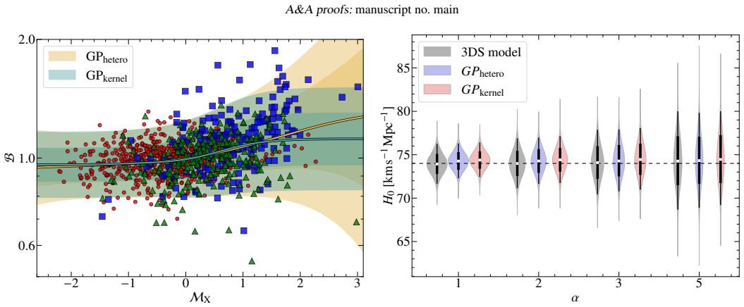
The central claim is that the cluster-structure bias B, which quantifies the mismatch between spectroscopic-like X-ray temperatures and temperatures reconstructed from the combination of millimetre and X-ray signals, is statistically predictable rather than an irreducible error. In a sample of 972 mock projections drawn from a hydrodynamical cluster simulation, B is positively skewed and leptokurtic, approximately log-normal overall but better described by three class-conditional log-normals (relaxed, hybrid, disturbed) or by Gaussian-process regressions against the X-ray morphological indicator MX. Injected into a Bayesian pipeline as informative priors, these descriptions produce H0 poster
Load-bearing premise
The B distribution measured from the redshift-zero snapshot of this hydrodynamical simulation is representative of real clusters at 0.05 < z < 0.6; if the simulated gas physics, morphology, or redshift evolution are unrealistic, the quoted unbiasedness, precision, and systematic floor do not transfer to real data.
Editorial extensions
If this is right
- A sample of 100 clusters yields about 4% precision on H0; 1000 clusters yield about 1.5%, with no significant mean bias in the mock tests.
- The variance scales as σ²(N) = σ0²/N + σs² with a non-zero systematic floor σs ≈ 0.6–0.8 km/s/Mpc, so beyond roughly 1200–1850 clusters additional clusters no longer improve H0.
- The probe is primarily an H0 probe: Ωm and the helium abundance are prior-dominated, and a 5% shift in the centres of those priors moves H0 by less than 1%.
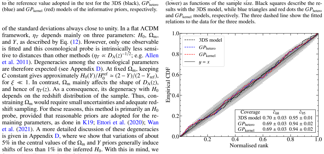
- Posterior calibration is close to nominal for all three prior models, supporting the use of the method on real data without ad hoc inflation of uncertainties.
- The morphology-dependent prior is statistically preferred over a single global distribution for B, so including dynamical-state information strengthens the analysis.
Reading between the lines
- Extension: because the mock catalogues draw B from the same simulation that provides the prior, the quoted unbiasedness is partly closed-loop; a decisive test is to apply the pipeline to observed clusters or to a simulation with different baryonic physics, where the paper itself flags that a residual dependence on the simulation model cannot be excluded.
- Extension: if the B–morphology relation holds in nature, morphology becomes a cheap conditioning variable, and H0 analyses need no longer throw away disturbed clusters; the useful sample for cluster standard-ruler cosmology would expand substantially.
- Extension: combining this probe, which scales as the inverse square root of angular diameter distance, with a probe scaling as a higher power of distance (for example gas fraction) could break the H0–helium degeneracy and let the same cluster data additionally constrain Ωm.
Editorial analysis
A structured set of objections, weighed in public.
Referee Report
Summary. This paper extends the Kozmanyan et al. (2019) X-ray/SZ 'standard-ruler' pipeline for H0 to a substantially larger simulation sample: 324 clusters from The300 gadget-x at z=0, projected along three lines of sight (972 mock objects). The cluster-structure bias B between X-ray spectroscopic-like and joint X-ray/SZ temperature reconstructions is measured from mock projected profiles, and its dependence on cluster dynamics/morphology is modelled in three ways: a single log-normal, a class-conditional mixture ('3DS', relaxed/hybrid/disturbed), and two Gaussian-process regressions against the X-ray morphology indicator MX. These distributions enter a Bayesian cosmological pipeline as informative priors — with analytic marginalisation over B (Eq. 27) — to infer H0 from mock ηT catalogues (Eq. 26) under flat ΛCDM with Planck-based priors on Ωm and Y. The pipeline is validated through 1000 bias realisations, a variance-scaling fit (σ² = σ0²/N + σs², with σ0 ≈ 26.6–26.9 km/s/Mpc and σs = 0.6–0.8), and simulation-based calibration (200 draws; 68%/95% coverage 0.69–0.70/0.94–0.95). Headline claims: unbiased H0 estimates with ~4% precision at N=100, ~1.5% at N=1000, and a systematic floor of 0.6–0.8 km/s/Mpc.
Significance. If the headline result holds, this is a valuable, careful step toward making cluster standard-ruler H0 constraints robust to ICM morphology, and a significant upgrade over K19 in sample size, in the morphology-aware priors, and above all in the rigour of the internal validation: LOS-length checks (App. A), projection-independence resampling with 10^6 draws (App. B), prior-sensitivity/disentanglement analyses (App. D), R-hat < 1.01 convergence, and a proper simulation-based calibration with reported 68%/95% coverage. Additional strengths are the analytic marginalisation of Eq. (27), the use of two GP implementations that agree where it matters, and the candid §5.1 disclosure of the residual dependence on the simulation model and the z=0 snapshot. The principal limitation is that the validation is closed-loop: the mock data are drawn from the same simulation sample that generates the priors, so the tests certify internal consistency but cannot bound the absolute accuracy of the B prior. Practical significance is therefore conditional; the quoted 0.6–0.8 km/s/Mpc 'ultimate' floor should not be read as the full systematic budget for real data.
major comments (1)
- [Abstract; §4.4.2–4.4.3; §5.1] The headline claims are established only in a closed loop: the mock catalogues of §4.4 (Eq. 26) draw ln B from the same 972-point gadget-x z=0 sample whose fitted log-normals (Table 1) and GP regressions (§4.3) define the informative priors (Table 2). The small MAP bias, the σs = 0.6–0.8 km/s/Mpc floor, and the SBC coverage therefore certify the pipeline's internal consistency given the prior; they cannot bound a global offset between the simulation's B distribution and that of real clusters. Because ln ηT = (1/2) ln H0 + ln B + const. (Eqs. 12–13), the quoted floor demands ~0.4% accuracy in the prior mean of ln B, and a constant offset δ in ln B would translate into a −2δ bias in ln H0 that no §4.4 test can detect. The §5.1 caveats are explicit but the abstract's 'unbiased' and 'ultimately limited by systematic uncertainties' are unconditional. Please qualify the headline claims and, pr
minor comments (8)
- [§3.3, Eq. (27)] For the GP models, μB and σB enter the marginal likelihood as the GP-predicted mean and scatter. Please state whether these are plug-in point predictions (e.g., posterior means) or whether GP predictive uncertainty is marginalised over. The SBC of §4.4.3 draws from the prior as implemented, so it checks calibration at fixed prior and does not test propagation of GP learning uncertainty; a short estimate of the GP posterior width of μ(MX) over the sampled MX range would settle the point.
- [§3.3, §4.4.2] The 3DS validation assigns clusters to classes with the 3D dynamical indicator χ, which is unavailable for observed clusters; in application the classes would have to come from morphological proxies, carrying the misclassification/projection risk the paper itself notes in §3.3. Since the 3DS and GP results agree, the impact is likely small, but please state explicitly how the 3DS prior is intended to be applied to real data and whether the class-conditional parameters are stable under the morphological (rather than 3D-dynamical) classification.
- [§4.4.2, Fig. 7] σ0 and σs are quoted without uncertainties. With only about six sample sizes in Fig. 7, the floor 0.6–0.8 km/s/Mpc — a headline number — has a non-negligible uncertainty; report confidence intervals for the fit parameters.
- [§4.4.1, Eq. (26)] Mock redshifts are drawn uniformly over 0.05–0.6. Since the H0–Ωm degeneracy depends on the redshift distribution (§4.4.1, App. D), the robustness of the quoted 4%/1.5% precision to a realistic, selection-driven redshift distribution (e.g., CHEX-MATE, which motivates the range) should be tested or justified.
- [§4.4.2] Please clarify the sampling details: are (B, MX) pairs for the GP mock catalogues drawn jointly from the 972-point sample with replacement, and are the 3DS class fractions fixed to the simulation values (57/25/18)? This matters for reproducing the variance-scaling numbers.
- [§5.1] The statement σMX ≲ 0.11 being 'well below' the GP length scales ℓµ ≃ 2, ℓσ ≃ 3 compares MX units with length scales on the Φ-transformed input x. Report the comparison in the transformed coordinate (δx ≃ δMX/σ(MX) at the peak of the normal density) or give the GP length scales in MX units.
- [Throughout] Proofreading: line-break artifacts such as 'di fferences' appear throughout the text, and the abstract has '1 .5%'. Also check author-name spacing in the reference list (e.g., 'V oit 2005'). A data/code availability statement for the PyMC and GP pipeline would support reproducibility.
- [§2, §5.1] The sample is high-mass-selected (median 7.7×10^14 M⊙). Although B is not significantly correlated with mass, a sentence in §5.1 on the expected portability of the B prior to lower-mass, survey-selected samples would strengthen the discussion of applicability.
Circularity Check
Partially circular validation: mock catalogues draw B from the same gadget-x z=0 sample used to build the informative B priors, so the quoted H0 unbiasedness and systematic floor are self-consistency results, with prior fidelity untested.
-
self definitional
[§4.4, Eq. (26); informative priors in Table 2 from fits in Table 1 and §4.3; limitation acknowledged in §5.1]
"For these tests, we generated mock ηmock T catalogues as follows. Given a sample size N, we randomly extracted B values from the simulated sample. … lnηmock T = ln h C(z; Href 0 , Ωref m , Yref) i + lnB +N(0, 0.14), (26)"
The mock catalogues draw ln B from the same 972-projection gadget-x z=0 sample whose empirical distribution is fitted in Table 1 and GP-regressed in §4.3, and these fits are exactly the informative priors in Table 2 (Bi ∼ LN(µi,σi), B(MX) ∼ LN[µGP,σGP]). Therefore the generative distribution for B is, by construction, the prior used in the inference. The resulting 'unbiased' H0 MAPs, the σ0 and σs ≈ 0.6–0.8 km/s/Mpc scaling, and the SBC coverage are prior-predictive self-consistency checks: they verify that the pipeline recovers parameters when the prior is correct, but cannot detect prior misspecification. The paper concedes: 'a residual dependence of the inferred B distribution on the adopted simulation model cannot be excluded,' so the headline precision/systematic floor is conditional
full rationale
Walked the derivation chain. The central load-bearing step is the §4.4 validation: mock ηT catalogues are generated with Eq. (26) by drawing B from the gadget-x z=0 sample, while the informative priors in Table 2 are the log-normal/GP fits to that same sample (§4.1, §4.3). Thus the validation measures posterior self-consistency under the assumption that the prior is exactly the true generative distribution. The reported unbiasedness, 4%/1.5% scaling, and 0.6–0.8 km/s/Mpc floor are conditional on that assumption and are not tests of the prior against real clusters. The paper itself states this in §5.1: residual simulation-model dependence 'cannot be excluded' and no explicit redshift-evolution test was made. I therefore flag this as partial circularity. However, the H0 part of the inference is not definitionally forced: H0 enters through C(z,ϑ), has a wide uniform prior, and the marginal-likelihood computation and variance scaling are nontrivial. The simulation's realism is also supported by external observational comparisons (Bartalucci et al. 2023; Campitiello et al. 2022; Rossetti et al. 2024; Lovisari et al. 2024), and the K19 self-citation is for the method being validated rather than an unverified uniqueness claim. Hence score 5, not higher.
Assumptions & free parameters
free parameters (5)
- Log-normal prior parameters (µ, σ) for B in each dynamical class =
µ: 1.08e-2 (single LN), -0.98e-2 (relaxed), -1.38e-2 (hybrid), 11.04e-2 (disturbed); σ: 13.29e-2, 9.68e-2, 13.28e-2, 18.
- GP kernel hyperparameters (amplitude, length scales, noise terms) =
ℓµ ≃ 2, ℓσ ≃ 3; other hyperparameters not fully reported
- σ0 and σs (statistical and systematic variance scaling) =
σ0 ≈ 26.6–26.9 km/s/Mpc; σs ≈ 0.6–0.8 km/s/Mpc
- Per-cluster log-normal noise (14%) =
14% (chosen)
- Reference mock cosmology (H0=74, Ωm=0.3153, Y=0.242) =
h_ref = 0.74, Ωm_ref = 0.3153, Y_ref = 0.242
assumptions (9)
- domain assumption ηT factorizes as bn·C·B with bn=1 in simulations (Eq. 11)
- domain assumption Vikhlinin et al. (2006) and Nagai et al. (2007) parametric profiles adequately describe projected ICM density, temperature, and pressure
- domain assumption Spectroscopic-like temperature weighting (Mazzotta et al. 2004) is the correct projection for X-ray temperature
- domain assumption Three orthogonal projections of the same 324 halos can be treated as independent objects
- domain assumption B is log-normally distributed
- domain assumption The gadget-x simulation of The300 reproduces the observed ICM properties needed for B
- domain assumption B does not evolve with redshift over 0.05 < z < 0.6
- standard math Gaussian likelihood for ln ηT and analytic marginalisation over ln B
- ad hoc to paper Gaussian priors on the class-conditional mean parameters µi, centred on the simulation-fit values
Cite this review
Pith. "Pith review of The Three Hundred Project: Validating $H_0$ inference from mock X-ray and millimetre analyses of galaxy clusters." pith.science (2026). https://pith.science/paper/MOGHPROE
@misc{pith2026260708613,
  author       = {Pith},
  title        = {Pith review of: The Three Hundred Project: Validating $H_0$ inference from mock X-ray and millimetre analyses of galaxy clusters},
  year         = {2026},
  howpublished = {\url{https://pith.science/paper/MOGHPROE}},
  note         = {Machine review of arXiv:2607.08613}
}
abstract
Measurements of thermodynamical quantities in galaxy clusters are differently affected by simplified modelling of radially averaged observables in the X-ray and millimetre bands. This includes assumptions about the cosmological model and the morphology of the cluster intracluster medium (ICM). Within a large sample of clusters extracted from The Three Hundred hydrodynamical simulations, we assess the systematic differences expected from the morphological assumptions between ICM temperatures as inferred from X-ray spectroscopy or joint X-ray and millimetre imaging. We find that these differences show a well-defined statistical behaviour that correlates with the cluster dynamical and morphological indicators. We then investigate how joint inferences of cluster temperature profiles, a priori informed by this statistical behaviour, allow us to constrain cosmological parameters inferred from the apparent cluster sizes. Assuming a flat $\Lambda$ cold dark matter ($\Lambda$CDM) cosmology and priors on $\Omega_\mathrm{m}$ and the helium abundance, this method provides us with unbiased estimates of the Hubble constant, $H_0$, characterised with a precision of about $4\%$ and $1.5\%$ for samples of 100 and 1000 clusters, respectively, and ultimately limited by systematic uncertainties of about $0.6$--$0.8\, {\rm km\, s^{-1} Mpc^{-1}}$. This work highlights the potential of joint X-ray and millimetre observations of galaxy cluster samples to place tight constraints on $H_0$.
Figures


Figures from the paper (3 more)

Reference graph
Works this paper leans on
-
[1]
2025, Phys
Abdul Karim, M., Aguilar, J., Ahlen, S., et al. 2025, Phys. Rev. D, 112, 083515
2025
-
[2]
2023, PeerJ Comput
Abril-Pla, O., Andreani, V ., Carroll, C., et al. 2023, PeerJ Comput. Sci., 9
2023
-
[3]
W., Evrard, A
Allen, S. W., Evrard, A. E., & Mantz, A. B. 2011, ARA&A, 49, 409
2011
-
[4]
Angulo, R. E. & Hahn, O. 2022, Living Rev. Comput. Astrophys., 8, 1
2022
-
[5]
2020, A&A, 634, A113
Ansarifard, S., Rasia, E., Biffi, V ., et al. 2020, A&A, 634, A113
2020
-
[6]
W., Piffaretti, R., et al
Arnaud, M., Pratt, G. W., Piffaretti, R., et al. 2010, A&A, 517, A92 Astropy Collaboration. 2013, A&A, 558, A33 Astropy Collaboration. 2018, AJ, 156, 123 Astropy Collaboration. 2022, ApJ, 935, 167
2010
-
[7]
W., Démoclès, J., & Lovisari, L
Bartalucci, I., Arnaud, M., Pratt, G. W., Démoclès, J., & Lovisari, L. 2019, A&A, 628, A86
2019
-
[8]
2023, A&A, 674, A179
Bartalucci, I., Molendi, S., Rasia, E., et al. 2023, A&A, 674, A179
2023
Show all 112 references
-
[9]
R., Pfrommer, C., & Sievers, J
Battaglia, N., Bond, J. R., Pfrommer, C., & Sievers, J. L. 2012, ApJ, 758, 74
2012
-
[10]
M., Murante, G., Arth, A., et al
Beck, A. M., Murante, G., Arth, A., et al. 2015, MNRAS, 455, 2110
2015
-
[11]
2012, MNRAS, 420, 3545
Biffi, V ., Dolag, K., Böhringer, H., & Lemson, G. 2012, MNRAS, 420, 3545
2012
-
[12]
1999, Phys
Birkinshaw, M. 1999, Phys. Rep., 310, 97
1999
-
[13]
E., et al
Bocquet, S., Grandis, S., Bleem, L. E., et al. 2024, Phys. Rev. D, 110, 083510 Böhringer, H., Dolag, K., & Chon, G. 2012, A&A, 539, A120 Böhringer, H. & Werner, N. 2010, A&A Rev., 18, 127
2024
-
[14]
K., LaRoque, S
Bonamente, M., Joy, M. K., LaRoque, S. J., et al. 2006, ApJ, 647, 25
2006
-
[15]
2017, ApJ, 843, 72
Bourdin, H., Mazzotta, P., Kozmanyan, A., Jones, C., & Vikhlinin, A. 2017, ApJ, 843, 72
2017
-
[16]
Buote, D. A. & Tsai, J. C. 1995, ApJ, 452, 522
1995
-
[17]
G., Ettori, S., Lovisari, L., et al
Campitiello, M. G., Ettori, S., Lovisari, L., et al. 2022, A&A, 665, A117
2022
-
[18]
E., Holder, G
Carlstrom, J. E., Holder, G. P., & Reese, E. D. 2002, ARA&A, 40, 643
2002
-
[19]
1979, A&A, 75, 322
Cavaliere, A., Danese, L., & de Zotti, G. 1979, A&A, 75, 322
1979
-
[20]
2025, A&A, 699, A141 CHEX-MATE Collaboration
Chappuis, L., Eckert, D., Sereno, M., et al. 2025, A&A, 699, A141 CHEX-MATE Collaboration. 2021, A&A, 650, A104
2025
-
[21]
2018, MNRAS, 477, 139
Cialone, G., De Petris, M., Sembolini, F., et al. 2018, MNRAS, 477, 139
2018
-
[22]
R., Gelman, A., & Rubin, D
Cook, S. R., Gelman, A., & Rubin, D. B. 2006, J. Comput. Graph. Stat., 15, 675
2006
-
[23]
Cowie, L. L. & Perrenod, S. C. 1978, ApJ, 219, 354
1978
-
[24]
M., Evrard, A
Crone, M. M., Evrard, A. E., & Richstone, D. O. 1996, ApJ, 467, 489
1996
-
[25]
Croton, D. J. 2013, PASA, 30, e052
2013
-
[26]
2022, MNRAS, 514, 977
Cui, W., Dave, R., Knebe, A., et al. 2022, MNRAS, 514, 977
2022
-
[27]
2018, MNRAS, 480, 2898
Cui, W., Knebe, A., Yepes, G., et al. 2018, MNRAS, 480, 2898
2018
-
[28]
2017, MNRAS, 464, 2502 De Luca, F., Bourdin, H., Mazzotta, P., et al
Cui, W., Power, C., Borgani, S., et al. 2017, MNRAS, 464, 2502 De Luca, F., Bourdin, H., Mazzotta, P., et al. 2026, A&A, 707, A32 De Luca, F., De Petris, M., Yepes, G., et al. 2021, MNRAS, 504, 5383 Di Valentino, E., Said, J. L., Riess, A., et al. 2025, Phys. Dark Universe, 49, 101965
2017
-
[29]
2015, MNRAS, 447, 2198
Eckert, D., Roncarelli, M., Ettori, S., et al. 2015, MNRAS, 447, 2198
2015
-
[30]
2013, Space Sci
Ettori, S., Donnarumma, A., Pointecouteau, E., et al. 2013, Space Sci. Rev., 177, 119
2013
-
[31]
2020, Astron
Ettori, S., Ghirardini, V ., & Eckert, D. 2020, Astron. Nachr, 341, 210
2020
-
[32]
2014, ApJ, 783, L10
Gaspari, M., Brighenti, F., Temi, P., & Ettori, S. 2014, ApJ, 783, L10
2014
-
[33]
2019, ApJ, 884, 169
Gaspari, M., Eckert, D., Ettori, S., et al. 2019, ApJ, 884, 169
2019
-
[34]
& Rubin, D
Gelman, A. & Rubin, D. B. 1992, Stat. Sci., 7, 457
1992
-
[35]
2024, A&A, 689, A298
Ghirardini, V ., Bulbul, E., Artis, E., et al. 2024, A&A, 689, A298
2024
-
[36]
2019, A&A, 621, A41
Ghirardini, V ., Eckert, D., Ettori, S., et al. 2019, A&A, 621, A41
2019
-
[37]
2022, MNRAS, 518, 4238
Gianfagna, G., Rasia, E., Cui, W., et al. 2022, MNRAS, 518, 4238
2022
-
[38]
J., Klein, M., & Dolag, K
Grandis, S., Bocquet, S., Mohr, J. J., Klein, M., & Dolag, K. 2021, MNRAS, 507, 5671
2021
-
[39]
2024, MNRAS, 532, 1031
Haggar, R., De Luca, F., De Petris, M., et al. 2024, MNRAS, 532, 1031
2024
-
[40]
E., Pearce, F
Haggar, R., Gray, M. E., Pearce, F. R., et al. 2020, MNRAS, 492, 6074
2020
-
[41]
R., Millman, K
Harris, C. R., Millman, K. J., van der Walt, S. J., et al. 2020, Nature, 585, 357–362
2020
-
[42]
Hastings, W. K. 1970, Biometrika, 57, 97
1970
-
[43]
A., Barnes, D
Henson, M. A., Barnes, D. J., Kay, S. T., McCarthy, I. G., & Schaye, J. 2017, MNRAS, 465, 3361
2017
-
[44]
Hoffman, M. D. & Gelman, A. 2014, J. Mach. Learn. Res., 15, 1593
2014
-
[45]
Hunter, J. D. 2007, Comput. Sci. Eng., 9, 90
2007
-
[46]
1986, MNRAS, 222, 323
Kaiser, N. 1986, MNRAS, 222, 323
1986
-
[47]
2008, ApJ, 674, 11
Kawahara, H., Kitayama, T., Sasaki, S., & Suto, Y . 2008, ApJ, 674, 11
2008
-
[48]
2024, A&A, 686, A97
Kim, J., Sayers, J., Sereno, M., et al. 2024, A&A, 686, A97
2024
-
[49]
2016, MNRAS, 457, 4340
Klypin, A., Yepes, G., Gottlöber, S., Prada, F., & Heß, S. 2016, MNRAS, 457, 4340
2016
-
[50]
Knollmann, S. R. & Knebe, A. 2009, ApJS, 182, 608
2009
-
[51]
2019, A&A, 621, A34
Kozmanyan, A., Bourdin, H., Mazzotta, P., Rasia, E., & Sereno, M. 2019, A&A, 621, A34
2019
-
[52]
Kravtsov, A. V . & Borgani, S. 2012, ARA&A, 50, 353
2012
-
[53]
V ., Vikhlinin, A., & Nagai, D
Kravtsov, A. V ., Vikhlinin, A., & Nagai, D. 2006, ApJ, 650, 128
2006
-
[54]
Kumar, R., Carroll, C., Hartikainen, A., & Martin, O. 2019, J. Open Source Softw., 4, 1143
2019
-
[55]
T., Hearin, A
Lau, E. T., Hearin, A. P., Nagai, D., & Cappelluti, N. 2020, MNRAS, 500, 1029
2020
-
[56]
T., Nagai, D., Avestruz, C., Nelson, K., & Vikhlinin, A
Lau, E. T., Nagai, D., Avestruz, C., Nelson, K., & Vikhlinin, A. 2015, ApJ, 806, 68
2015
-
[57]
2023, MNRAS, 523, 1228
Li, Q., Cui, W., Yang, X., et al. 2023, MNRAS, 523, 1228
2023
-
[58]
2020, MNRAS, 495, 2930 Article number, page 11 of 16 A&A proofs: manuscript no
Li, Q., Cui, W., Yang, X., et al. 2020, MNRAS, 495, 2930 Article number, page 11 of 16 A&A proofs: manuscript no. aa60643-26
2020
-
[59]
2024, A&A, 682, A45
Lovisari, L., Ettori, S., Rasia, E., et al. 2024, A&A, 682, A45
2024
-
[60]
V ., Dutton, A
Maccio, A. V ., Dutton, A. A., Van Den Bosch, F. C., et al. 2007, MNRAS, 378, 55
2007
-
[61]
H., Clowe, D., et al
Markevitch, M., Gonzalez, A. H., Clowe, D., et al. 2004, ApJ, 606, 819
2004
-
[62]
E., & Mohr, J
Mathiesen, B., Evrard, A. E., & Mohr, J. J. 1999, ApJ, 520, L21
1999
-
[63]
2004, MNRAS, 354, 10
Mazzotta, P., Rasia, E., Moscardini, L., & Tormen, G. 2004, MNRAS, 354, 10
2004
-
[64]
W., Bayliss, M., et al
McDonald, M., Allen, S. W., Bayliss, M., et al. 2017, ApJ, 843, 28
2017
-
[65]
2010, in Proceedings of the 9th Python in Science Conference, ed
McKinney, W. 2010, in Proceedings of the 9th Python in Science Conference, ed. S. van der Walt & J. Millman, 56 – 61
2010
-
[66]
2010, A&A, 514, A93
Meneghetti, M., Rasia, E., Merten, J., et al. 2010, A&A, 514, A93
2010
-
[67]
W., Rosenbluth, M
Metropolis, N., Rosenbluth, A. W., Rosenbluth, M. N., Teller, A. H., & Teller, E. 1953, J. Chem. Phys., 21, 1087
1953
-
[68]
2024, A&A, 688, A107
Migkas, K., Kox, D., Schellenberger, G., et al. 2024, A&A, 688, A107
2024
-
[69]
2026, in Encyclopedia of Astrophysics (First Edition), first edition edn., ed
Miyatake, H. 2026, in Encyclopedia of Astrophysics (First Edition), first edition edn., ed. I. Mandel (Oxford: Elsevier), 410–430
2026
-
[70]
J., Fabricant, D
Mohr, J. J., Fabricant, D. G., & Geller, M. J. 1993, ApJ, 413, 492
1993
-
[71]
V ., & Vikhlinin, A
Nagai, D., Kravtsov, A. V ., & Vikhlinin, A. 2007, ApJ, 668, 1
2007
-
[72]
Neal, R. M. 2003, Ann. Stat., 31, 705
2003
-
[73]
F., Gao, L., Bett, P., et al
Neto, A. F., Gao, L., Bett, P., et al. 2007, MNRAS, 381, 1450
2007
-
[74]
2010, A&A, 523, A22
Nevalainen, J., David, L., & Guainazzi, M. 2010, A&A, 523, A22
2010
-
[75]
A., et al
Nurgaliev, D., McDonald, M., Benson, B. A., et al. 2017, ApJ, 841, 5 Pandas development team. 2020, pandas-dev/pandas: Pandas
2017
-
[76]
Pedregosa, F., Varoquaux, G., Gramfort, A., et al. 2011, J. Mach. Learn. Res., 12, 2825 Planck Collaboration VI. 2020, A&A, 641, A6 Planck Collaboration XIII. 2016, A&A, 594, A13 Planck Collaboration XXIV. 2016, A&A, 594, A24
2011
-
[77]
Planelles, S., Schleicher, D. R. G., & Bykov, A. M. 2015, Space Sci. Rev., 188, 93
2015
-
[78]
W., Arnaud, M., Biviano, A., et al
Pratt, G. W., Arnaud, M., Biviano, A., et al. 2019, Space Sci. Rev., 215, 25
2019
-
[79]
2015, ApJ, 813, L17
Rasia, E., Borgani, S., Murante, G., et al. 2015, ApJ, 813, L17
2015
-
[80]
2013, Astron
Rasia, E., Meneghetti, M., & Ettori, S. 2013, Astron. Rev., 8, 40
2013
-
[81]
2012, New J
Rasia, E., Meneghetti, M., Martino, R., et al. 2012, New J. Phys., 14, 055018
2012
-
[82]
2025, A&A, 702, A182
Rasia, E., Tripodi, R., Borgani, S., et al. 2025, A&A, 702, A182
2025
-
[83]
Rasmussen, C. E. & Williams, C. K. I. 2005, Gaussian Processes for Machine Learning (The MIT Press)
2005
-
[84]
Reese, E. D. 2004, in Measuring and Modeling the Universe, ed. W. L. Freed- man, 138
2004
-
[85]
D., Kawahara, H., Kitayama, T., et al
Reese, E. D., Kawahara, H., Kitayama, T., et al. 2010, ApJ, 721, 653
2010
-
[86]
2013, MNRAS, 432, 3030
Roncarelli, M., Ettori, S., Borgani, S., et al. 2013, MNRAS, 432, 3030
2013
-
[87]
2024, A&A, 686, A68
Rossetti, M., Eckert, D., Gastaldello, F., et al. 2024, A&A, 686, A68
2024
-
[88]
2017, MNRAS, 468, 1917
Rossetti, M., Gastaldello, F., Eckert, D., et al. 2017, MNRAS, 468, 1917
2017
-
[89]
S., Rosati, P., Tozzi, P., et al
Santos, J. S., Rosati, P., Tozzi, P., et al. 2008, A&A, 483, 35
2008
-
[90]
S., Tozzi, P., Rosati, P., & Böhringer, H
Santos, J. S., Tozzi, P., Rosati, P., & Böhringer, H. 2010, A&A, 521, A64
2010
-
[91]
J., Crampton, D., et al
Schade, D., Lilly, S. J., Crampton, D., et al. 1995, ApJ, 451
1995
-
[92]
H., Lovisari, L., Nevalainen, J., & David, L
Schellenberger, G., Reiprich, T. H., Lovisari, L., Nevalainen, J., & David, L. 2015, A&A, 575, A30
2015
-
[93]
W., Allen, S
Schmidt, R. W., Allen, S. W., & Fabian, A. C. 2004, MNRAS, 352, 1413
2004
-
[94]
2012, MNRAS, 429, 323
Sembolini, F., Yepes, G., De Petris, M., et al. 2012, MNRAS, 429, 323
2012
-
[95]
2018, ApJ, 860, L4
Sereno, M., Umetsu, K., Ettori, S., et al. 2018, ApJ, 860, L4
2018
-
[96]
& White, S
Silk, J. & White, S. D. M. 1978, ApJ, 226, L103
1978
-
[97]
2005, MNRAS, 364, 1105
Springel, V . 2005, MNRAS, 364, 1105
2005
-
[98]
Sulkanen, M. E. 1999, ApJ, 522, 59
1999
-
[99]
2024, Phys
Sunayama, T., Miyatake, H., Sugiyama, S., et al. 2024, Phys. Rev. D, 110, 083511
2024
-
[100]
Sunyaev, R. A. & Zeldovich, I. B. 1980, ARA&A, 18, 537
1980
-
[101]
Sunyaev, R. A. & Zeldovich, Y . B. 1972, Com. Ap&SS, 4, 173
1972
-
[102]
2018, arXiv e-prints, arXiv:1804.06788
Talts, S., Betancourt, M., Simpson, D., Vehtari, A., & Gelman, A. 2018, arXiv e-prints, arXiv:1804.06788
2018 arXiv
-
[103]
2018, MNRAS, 474, 4089
Truong, N., Rasia, E., Mazzotta, P., et al. 2018, MNRAS, 474, 4089
2018
-
[104]
2021, Bayesian Anal., 16, 667
Vehtari, A., Gelman, A., Simpson, D., Carpenter, B., & Bürkner, P.-C. 2021, Bayesian Anal., 16, 667
2021
-
[105]
2006, ApJ, 640, 691
Vikhlinin, A., Kravtsov, A., Forman, W., et al. 2006, ApJ, 640, 691
2006
-
[106]
V ., Burenin, R
Vikhlinin, A., Kravtsov, A. V ., Burenin, R. A., et al. 2009, ApJ, 692, 1060
2009
-
[107]
E., et al
Virtanen, P., Gommers, R., Oliphant, T. E., et al. 2020, Nat. Methods, 17, 261 V ogelsberger, M., Marinacci, F., Torrey, P., & Puchwein, E. 2020, Nat. Rev. Phys., 2, 42 V oit, G. M. 2005, Rev. Mod. Phys., 77, 207
2020
-
[108]
T., Mantz, A
Wan, J. T., Mantz, A. B., Sayers, J., et al. 2021, MNRAS, 504, 1062
2021
-
[109]
Waskom, M. L. 2021, J. Open Source Softw., 6, 3021
2021
-
[110]
H., Mortonson, M
Weinberg, D. H., Mortonson, M. J., Eisenstein, D. J., et al. 2013, Phys. Rep., 530, 87
2013
-
[111]
A., Bi ffi, V ., Hallman, E
ZuHone, J. A., Bi ffi, V ., Hallman, E. J., et al. 2014, in Proceedings of the 13th Python in Science Conference, ed. S. van der Walt & J. Bergstra, 98–104
2014
-
[112]
ZuHone, J. A. & Hallman, E. J. 2016, pyXSIM: Synthetic X-ray observations generator Article number, page 12 of 16 F. De Luca et al.: The300 Project: Validating H0 inference from mock X-ray and millimetre analyses of galaxy clusters Appendix A: Dependence on LOS integration 0.5...
2016
Reviewed August 2, 2026 · model on record in the stance chip above.
Discussion (0). Sign in to comment.