REVIEW 3 major objections 5 minor 47 references
Near-Field Sampling for Line Sources
T0 review · 3 major / 5 minor · reviewed 2026-08-01 · deepseek-v4-flash
Pith's one-line read Near-field sampling for line sources reaches the SVD-optimal bound using geometry alone.
desk verdict Solid geometry-based sampling scheme; the propagating-mode part is a genuine contribution, but the post-knee reactive gain leans on a parameter picked post hoc, so the outperformance claim needs robustness tests. read the letter →
The pith
A machine-rendered reading of the paper's core claim, the machinery that carries it, and where it could break.
The reading
What carries the argument
View-length DoF density: ρ_p(r_R) = (1/λ) ∫_{Tx} |(lhat_T×R)·(lhat_R×R)|/|R|³ dl_T, whose cumulative integral L_TR defines the 'DoF coordinate' in which uniform spacing means one sample per DoF. This density is the mechanism that maps geometry to sampling locations; it gives the total mode count, the local concentration of propagating modes, and the one-DoF placement rule (13). The reactive correction is a power-law weight q_r(f)=f^{-p}+(1−f)^{-p} in that same coordinate, used only after the knee to concentrate extra samples at the receiver ends. The error functional E(P_N)=||H(eH†eH−I)||_2=||Σ(V^H eV eV^H V−I)||_2 provides the Eckart–Young lower bound that the scheme is calibrated against.
What would settle it
Compute the channel singular values for a line pair with strong curvature or a near-90° receiver bend (the paper's own 'excessive bending' caveat), and compare the spectral transition to ⌈L_TR/λ⌉ from (11); a mismatch beyond a few modes would place the view-length count on the wrong side for 3D curves. A cleaner check: on any tested geometry, plot E(P_N) with the reactive term removed—if the gap to σ_{N+1}/σ1 fails to close as N grows, the reactive-density model is not the right correction.
Extended reading notes
Core claim
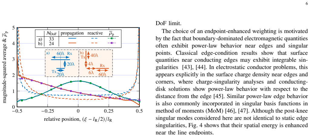
Near-field samples for line sources can be chosen directly from geometry. The paper's central claim is that the number and placement of significant spatial modes are governed by the view length between the source and receiver curves, L_TR = ∫∫ |(lhat_T×R)·(lhat_R×R)|/|R|³ dl_R dl_T, with NDoF = L_TR/λ. Sampling at points ξ_n satisfying L_TR(ξ_{n+1})−L_TR(ξ_n)=λ (one sample per degree of freedom) captures the dominant propagating subspace; beyond the NDoF knee, additional samples are placed according to the reactive density ρ_r ∝ [f(ξ)^{-p}+(1−f(ξ))^{-p}]ρ_p(ξ) with p=2/3, where f is the DoF-normalized cumulative coordinate. The sampling error E(P_N) is shown to be at least σ_{N+1}, the first
Load-bearing premise
The load-bearing assumption is that one geometric integral—the view length between the source and receiver lines—continues to count the spatial modes correctly when the lines are non-coplanar or gently curved in 3D; if that count is wrong, the knee location and every sampling point derived from it shift.
Editorial extensions
If this is right
- For line-source/receiver geometries, the number of significant samples can be set by NDoF = L_TR/λ and the locations read off from one cumulative integral, without building the channel matrix.
- Sampling schemes that use only the propagating DoF density will converge slowly after the spectral knee; the reactive edge density is needed to match the SVD bound.
- The error of any N-point near-field sample set is at least the (N+1)-th singular value, so a good sampling rule should target that bound; the proposed rule does so in the tested geometries.
- The placement rule transfers across parallel, perpendicular, rotated, non-coplanar, and moderately curved configurations, suggesting it depends only on the view-length structure, not on coordinate-system details.
- In antenna measurement/inverse-source settings, this implies geometry-adaptive nonuniform sampling grids can replace dense uniform grids while preserving dominant modes.
Reading between the lines
- If the view-length count also holds for two-dimensional surfaces (a suggested future direction), the same one-DoF placement idea would become a surface sampling rule, potentially unifying near-field sampling, beamforming, and inverse-source discretization under one geometric functional.
- The reactive power-law exponent p=2/3 is chosen empirically from two examples; an editorial extension would be to test whether p depends on edge geometry, source length, or separation, or whether an adaptive estimator of post-knee mode energy could replace the fixed exponent.
- The scalar Green's function idealization leaves polarization coupling and multiple field components unexplored; if the vector extension preserves the density interpretation, the sampling rule could be applied directly to full electromagnetic measurements.
- A practical near-field measurement campaign could validate the rule by comparing reconstruction error against uniform sampling with the same sample count; the paper's numerical setup offers a ready protocol for such a test.
Editorial analysis
A structured set of objections, weighed in public.
Referee Report
Summary. The paper develops a geometry-aware sampling framework for near-field line-source systems. Starting from a scalar Green's-function channel model, it defines a sampling error functional (7) and proves that it is lower-bounded by the first neglected singular value of the dense channel (8). It then derives a propagating-mode DoF density from the view-length (mutual-shadow) integral (11), uses equal increments of the cumulative density to place one-DoF samples (13), and augments this with a heuristic reactive-mode density (23)-(25) to improve post-knee sampling. Numerical experiments for parallel, perpendicular, non-coplanar, and gently curved line pairs compare the proposed strategy against uniform, DoF-center, DoF-edge, DEIM, and the singular-value bound, reporting that the method closely tracks the SVD-optimal performance and outperforms propagating-only sampling.
Significance. If the claims are robust, the framework offers a computationally cheap, geometry-driven alternative to matrix-based sample selection (e.g., DEIM) for near-field line sampling, with a rigorous operator-side error bound. The derivation of the propagating density as the total variation of the projected-direction function (17)-(19) is clean and elegant, and the numerical validation spans a wider set of 3D geometries than is often considered. However, two load-bearing points need attention before the claims can be fully accepted: the 3D view-length formula (11) is asserted without derivation, and the reactive-density exponent p=2/3 is selected post hoc on the same benchmark used to demonstrate the method's advantage.
major comments (3)
- [Sec. III-B, Eq. (11), and Sec. IV] The 3D view-length formula (11) is carried over from the 2D mutual-shadow result (9) without a derivation. The manuscript itself states, 'The generalized expression (11) for curves in R^3 is validated numerically in Sec. IV.' Since (11) feeds directly into the density (14)-(20), the one-DoF rule (13), and the knee location for all non-coplanar and curved examples, its status is load-bearing. The scope caveat 'provided that the curves do not exhibit excessive bending' is heuristic. Please either derive (11) from a local-tangent/infinitesimal-segment argument and state the regime of validity, or explicitly label it as a conjecture supported by numerical evidence. The conclusion's phrase 'closed-form expressions were derived' overstates the current state.
- [Sec. III-C, Eqs. (23)-(25), and Fig. 5] The reactive-density exponent p=2/3 is selected post hoc on the same benchmark used to support the central outperformance claim: 'Among the tested choices, p=2/3 provides the clearest improvement and is therefore used in all examples throughout this paper.' Only p=0.5 and p=2/3 are shown, so the sensitivity to this free parameter is not established. Since the abstract's 'significantly outperforms' claim is specifically about the post-knee reactive correction, add a p-sweep for representative configurations, derive p from the edge-condition asymptotics of the Helmholtz operator, or otherwise show that the improvement is robust over a range of p. Without this, the claim could be an artifact of a favorable parameter choice.
- [Sec. III-A, Eq. (13) and DoF-edge/DoF-center definitions] The one-DoF condition (13) equates a cumulative view-length increment to exactly one wavelength, which for integer NDoF would imply NDoF+1 sample points (including both endpoints). The implementation instead uses N points with equal increments in the DoF coordinate, giving N-1 intervals for DoF-edge and N cells for DoF-center. The manuscript says 'the sampling intervals are adjusted... so that each cell represents approximately NDoF/N spatial DoF,' which is not the same as (13). This ambiguity affects the x-axis interpretation in Figs. 2 and 5-8 and the 'one-DoF' terminology. Please define exactly how N maps to the point set (N intervals vs. N-1 intervals, inclusion of endpoints) for each sampling rule.
minor comments (5)
- [Sec. II, Eq. (8)] The norm equality in (8) uses the unitarity of V^H; this step is not explicitly stated. A one-line justification would improve readability.
- [App. A, Eqs. (29) and (31)] The expressions (29) and (31) are view-length densities, whereas the DoF density in (20) includes a factor 1/λ. Please state explicitly whether the Appendix expressions omit this factor and note that the normalization in Sec. III-C cancels it.
- [General] The terms 'gently curved' (Sec. III) and 'monotone smoothly varying' (Sec. V) are used inconsistently; unify the terminology.
- [Fig. 4] The caption says 'following 25 reactive modes,' but the text in Sec. III-C mentions the first 25 post-knee modes. Clarify the definition.
- [Eqs. (5)-(6)] The reconstructed field is denoted bER in (5) but the error in (6) is written as bER - E_R; define bER explicitly as the reconstructed dense-field vector.
Circularity Check
Reactive exponent p=2/3 is selected post hoc on the same benchmark used to demonstrate outperformance, making the headline quantitative claim partially in-sample.
-
fitted input called prediction
[Section III-C, paragraph following Fig. 5 (Eqs. (23)-(25))]
"Among the tested choices, p=2/3 provides the clearest improvement and is therefore used in all examples throughout this paper."
The reactive density (25), which is the source of the post-knee outperformance claimed in the abstract, contains an exponent p that is not derived from edge-condition asymptotics but selected by inspecting the very Fig. 5 sampling-error curves that are then presented as evidence. With no p-sensitivity analysis, the p=2/3 curves demonstrate a tuned fit rather than a parameter-free prediction; the same benchmark cannot independently validate a parameter chosen to improve on it. The paper further states that the reactive-integral benchmark, built from the post-knee singular modes, gives even more improvement, confirming that p=2/3 is a fitted approximation rather than a derived consequence.
full rationale
The propagating-mode part of the derivation is not circular: Eq. (8) is an Eckart-Young lower bound, the DoF density (20) follows from the view-length formulation of [27], and the one-DoF placement rule is benchmarked against dense-channel SVD and DEIM, giving independent, falsifiable references. Self-citations [27], [37], and [41] are present, but the central sampling-error comparisons are anchored to the dense-channel singular-value spectrum, so they are not solely load-bearing. The genuine circularity is restricted to the reactive component: q_r(f) is an unmotivated power-law ansatz, and the exponent p=2/3 is chosen after examining the same Fig. 5 data used to support the abstract's 'closely approaches' and 'significantly outperforms' claims. Because p=0.5 also improves over DoF-edge sampling, the qualitative effect is not entirely manufactured, but the quantitative headline claim is partly an in-sample consequence of parameter selection. Hence score 5: partial circularity with the central propagating derivation retaining independent content.
Assumptions & free parameters
free parameters (3)
- Reactive-density exponent p =
p = 2/3
- Number of post-knee modes in diagnostic benchmark =
25 modes ("at least 75% of the identified reactive modes")
- Dense reference grid spacing =
λ/50
assumptions (6)
- domain assumption Scalar propagation model: E(r_R) = ∫ G(r_R, r_T) J(r_T) dl_T with scalar Green's function, one field component
- domain assumption NDoF = L_TR/λ, the view-length (mutual-shadow) degrees-of-freedom estimate
- ad hoc to paper 3D generalization (11): for curves in R³ the view length is ∫∫ |(l̂_T×R)·(l̂_R×R)|/|R|³ dl_R dl_T
- domain assumption Full mutual visibility without occlusion; gently curved lines with gradually varying tangent directions
- domain assumption Singular-value spectrum separates into propagating, reactive, and noise-dominated regions (spectral knee)
- standard math Eckart–Young theorem: best rank-N approximation error of H is σ_{N+1}
Cite this review
Pith. "Pith review of Near-Field Sampling for Line Sources." pith.science (2026). https://pith.science/paper/YUD2WFYZ
@misc{pith2026260720701,
  author       = {Pith},
  title        = {Pith review of: Near-Field Sampling for Line Sources},
  year         = {2026},
  howpublished = {\url{https://pith.science/paper/YUD2WFYZ}},
  note         = {Machine review of arXiv:2607.20701}
}
read the original abstract
Near-field sampling seeks to represent electromagnetic fields between transmitting and receiving regions using a minimal number of measurement points while preserving the dominant spatial modes. This paper develops a geometry-aware sampling framework based on spatial degrees of freedom (DoF). A view-length formulation is used to derive closed-form expressions for the propagating-mode DoF density for simple line-source geometries, providing both the total DoF and its local distribution. One-DoF sampling points are obtained from equal increments of the cumulative DoF density, yielding an adaptive nonuniform sampling strategy up to the knee of the singular-value spectrum. To improve the representation of the remaining modes beyond the knee, a reactive-mode density is introduced to guide the placement of additional edge samples. An operator-based sampling error functional is formulated and shown to be lower-bounded by the neglected singular values of the continuous channel operator. Numerical results demonstrate that the proposed sampling strategy closely approaches the optimal performance obtained from singular-value decomposition and significantly outperforms sampling based solely on the propagating-mode DoF density.
Figures


Figures from the paper (4 more)


Reference graph
Works this paper leans on
-
[1]
Efficient near-field far-field transformation for nonredundant sampling representation on arbitrary surfaces in near-field antenna measurements,
M. A. Qureshi, C. H. Schmidt, and T. F. Eibert, “Efficient near-field far-field transformation for nonredundant sampling representation on arbitrary surfaces in near-field antenna measurements,”IEEE Trans. Antennas Propag., vol. 61, no. 4, pp. 2025–2033, Dec. 2012
2025
-
[2]
Antenna characterization from a small number of far-field measurements via reduced-order models,
N. M ´ezi`eres, M. Mattes, and B. Fuchs, “Antenna characterization from a small number of far-field measurements via reduced-order models,” IEEE Trans. Antennas Propag., vol. 70, no. 4, pp. 2422–2430, Oct. 2021
2021
-
[3]
Fast antenna far-field characterization via sparse spherical harmonic expansion,
B. Fuchs, L. Le Coq, S. Rondineau, and M. D. Migliore, “Fast antenna far-field characterization via sparse spherical harmonic expansion,”IEEE Trans. Antennas Propag., vol. 65, no. 10, pp. 5503–5510, Aug. 2017
2017
-
[4]
Singular value optimization in inverse electromagnetic scattering,
A. Capozzoli, C. Curcio, and A. Liseno, “Singular value optimization in inverse electromagnetic scattering,”IEEE Antennas Wireless Propag. Lett., vol. 16, pp. 1094–1097, Dec. 2016
2016
-
[5]
A two-step inverse-scattering technique in variable- exponent lebesgue spaces for through-the-wall microwave imaging: Experimental results,
A. Randazzoet al., “A two-step inverse-scattering technique in variable- exponent lebesgue spaces for through-the-wall microwave imaging: Experimental results,”IEEE Trans. Geosci. Remote Sens., vol. 59, no. 9, pp. 7189–7200, Sep. 2021
2021
-
[6]
Near-field transverse reso- lution in planar source reconstructions,
M. A. Maisto, R. Pierri, and R. Solimene, “Near-field transverse reso- lution in planar source reconstructions,”IEEE Trans. Antennas Propag., vol. 69, no. 8, pp. 4836–4845, Aug. 2021
2021
-
[7]
Inverse source problem and minimum-energy sources,
E. A. Marengo, A. J. Devaney, and R. W. Ziolkowski, “Inverse source problem and minimum-energy sources,”J. Opt. Soc. Amer . A, vol. 17, no. 1, pp. 34–45, 2000
2000
-
[8]
Reactive near-field reconstruction via Rayleigh–Sommerfeld integral: Ill-conditioning analysis and regulariza- tion,
D.-H. Han and X.-C. Wei, “Reactive near-field reconstruction via Rayleigh–Sommerfeld integral: Ill-conditioning analysis and regulariza- tion,”IEEE Trans. Microw. Theory Techn., pp. 1–10, 2026
2026
Show all 47 references
-
[9]
Inverse source in the near field: The case of a strip current,
R. Solimene, M. A. Maisto, and R. Pierri, “Inverse source in the near field: The case of a strip current,”J. Opt. Soc. Amer . A., vol. 35, no. 5, pp. 755–763, 2018
2018
-
[10]
Electromagnetic inverse scattering: Re- trievable information and measurement strategies,
O. M. Bucci and T. Isernia, “Electromagnetic inverse scattering: Re- trievable information and measurement strategies,”Radio Sci., vol. 32, no. 6, pp. 2123–2137, 1997
1997
-
[11]
An overview of near-field antenna measurements,
A. Yaghjian, “An overview of near-field antenna measurements,”IEEE Trans. Antennas Propag., vol. 34, no. 1, pp. 30–45, Jan. 1986
1986
-
[12]
R. J. Marks II,Advanced Topics in Shannon Sampling and Interpolation Theory. New York, NY , USA: Springer-Verlag, 1993
1993
-
[13]
Communicating with waves between volumes: Evaluating orthogonal spatial channels and limits on coupling strengths,
D. A. Miller, “Communicating with waves between volumes: Evaluating orthogonal spatial channels and limits on coupling strengths,”Appl. Opt., vol. 39, no. 11, pp. 1681–1699, Apr. 2000
2000
-
[14]
IV light and information,
D. Gabor, “IV light and information,” inProgress in Optics, vol. 1. Amsterdam, The Netherlands: Elsevier, 1961, pp. 109–153
1961
-
[15]
On the degrees of freedom of scattered fields,
O. M. Bucci and G. Franceschetti, “On the degrees of freedom of scattered fields,”IEEE Trans. Antennas Propag., vol. 37, no. 7, pp. 918– 926, Jul. 1989
1989
-
[16]
Franceschetti,Wave Theory of Information
M. Franceschetti,Wave Theory of Information. Cambridge, U.K.: Cambridge Univ. Press, 2017
2017
-
[17]
Degrees of freedom and sampling representation of electromagnetic fields: Concepts and applications
O. M. Bucci and M. D. Migliore, “Degrees of freedom and sampling representation of electromagnetic fields: Concepts and applications.” IEEE Antennas Propag. Mag., vol. 67, no. 3, pp. 10–22, Jun. 2025
2025
-
[18]
Degrees of freedom in multiple-antenna channels: A signal space approach,
A. S. Poon, R. W. Brodersen, and D. N. Tse, “Degrees of freedom in multiple-antenna channels: A signal space approach,”IEEE Trans. Inf. Theory, vol. 51, no. 2, pp. 523–536, Feb. 2005
2005
-
[19]
Communicating with large intelligent surfaces: Fundamen- tal limits and models,
D. Dardari, “Communicating with large intelligent surfaces: Fundamen- tal limits and models,”IEEE J. Sel. Areas Commun., vol. 38, no. 11, pp. 2526–2537, Nov. 2020
2020
-
[20]
Capacity of the continuous-space electromagnetic channel,
M. A. Jensen and J. W. Wallace, “Capacity of the continuous-space electromagnetic channel,”IEEE Trans. Antennas Propag., vol. 56, no. 2, pp. 524–531, Feb. 2008
2008
-
[21]
Maximizing independent channels and efficiency in BTS array antennas via EM degrees of freedom,
F. Puggelli, B. Biscontini, E. Martini, and S. Maci, “Maximizing independent channels and efficiency in BTS array antennas via EM degrees of freedom,”IEEE Trans. Antennas Propag., vol. 73, no. 6, pp. 3444–3458, Jun. 2025
2025
-
[22]
Breaking the degrees-of-freedom limit of holo- graphic MIMO communications: A 3-D antenna array topology,
S. S. A. Yuan et al., “Breaking the degrees-of-freedom limit of holo- graphic MIMO communications: A 3-D antenna array topology,”IEEE Trans. V eh. Technol., vol. 73, no. 8, pp. 11 276–11 288, Aug. 2024
2024
-
[23]
Arendt, R
W. Arendt, R. Nittka, W. Peter, and F. Steiner,Weyl’s Law: Spectral Properties of the Laplacian in Mathematics and Physics. John Wiley & Sons, Ltd, 2009
2009
-
[24]
Representation of elec- tromagnetic fields over arbitrary surfaces by a finite and nonredundant number of samples,
O. M. Bucci, C. Gennarelli, and C. Savarese, “Representation of elec- tromagnetic fields over arbitrary surfaces by a finite and nonredundant number of samples,”IEEE Trans. Antennas Propag., vol. 46, no. 3, pp. 351–359, Mar. 1998
1998
-
[25]
Waves, modes, communications, and optics: A tutorial,
D. A. Miller, “Waves, modes, communications, and optics: A tutorial,” Adv. Opt. Photon., vol. 11, no. 3, pp. 679–825, 2019
2019
-
[26]
Electromagnetic degrees of freedom of an optical system,
R. Piestun and D. A. Miller, “Electromagnetic degrees of freedom of an optical system,”JOSA A, vol. 17, no. 5, pp. 892–902, 2000
2000
-
[27]
Shadow area and degrees of freedom for free-space communication,
M. Gustafsson, “Shadow area and degrees of freedom for free-space communication,”IEEE J. Sel. Areas Inf. Theory, vol. 6, pp. 325–337, 2025
2025
-
[28]
Degrees of freedom for radiating systems,
——, “Degrees of freedom for radiating systems,”IEEE Trans. Antennas Propag., vol. 73, no. 2, pp. 1028–1038, Feb. 2025
2025
-
[29]
Efficient planar near-field measurements for radiation pattern evaluation by a warping strategy,
M. A. Maisto, G. Leone, A. Brancaccio, and R. Solimene, “Efficient planar near-field measurements for radiation pattern evaluation by a warping strategy,”IEEE Access, vol. 9, pp. 62 255–62 265, Apr. 2021
2021
-
[30]
Asymptotic study of the radiation operator for the strip current in near zone,
R. Pierri and R. Moretta, “Asymptotic study of the radiation operator for the strip current in near zone,”Electronics, vol. 9, no. 6, p. 911, May, 2020
2020
-
[31]
NDF of the near-zone field on a line perpendicular to the source,
——, “NDF of the near-zone field on a line perpendicular to the source,” IEEE Access, vol. 9, pp. 91 649–91 660, Jun. 2021
2021
-
[32]
Dimension and sampling of the near-field and its intensity over curves,
G. Leone, R. Moretta, and R. Pierri, “Dimension and sampling of the near-field and its intensity over curves,”IEEE Open J. Antennas Propag., vol. 3, pp. 412–424, Feb. 2022
2022
-
[33]
Sampling approach for singular system computation of a radiation operator,
R. Solimene, M. A. Maisto, and R. Pierri, “Sampling approach for singular system computation of a radiation operator,”J. Opt. Soc. Amer . A., vol. 36, no. 3, pp. 353–361, 2019
2019
-
[34]
An intuitive approach to the optimal sampling of an electromagnetic field,
M. D. Migliore, “An intuitive approach to the optimal sampling of an electromagnetic field,”Sensors, vol. 25, no. 24, p. 7591, 2025. 10
2025
-
[35]
An introduction to compressive sampling,
E. J. Cand `es and M. B. Wakin, “An introduction to compressive sampling,”IEEE Signal Process. Mag., vol. 25, no. 2, pp. 21–30, Mar. 2008
2008
-
[36]
Optimizing sensing matrices for spherical near-field antenna measurements,
A. Bangun and C. Culotta-L ´opez, “Optimizing sensing matrices for spherical near-field antenna measurements,”IEEE Trans. Antennas Propag., vol. 71, no. 2, pp. 1716–1724, Dec, 2022
2022
-
[37]
Interpreting moment matrix blocks spectra using mutual shadow area,
Y . Brick, F. P. Andriulli, and M. Gustafsson, “Interpreting moment matrix blocks spectra using mutual shadow area,”IEEE Trans. Antennas Propag., pp. 1–1, 2026
2026
-
[38]
Ben-Israel and T
A. Ben-Israel and T. Greville,Generalized Inverses: Theory and Appli- cations. New York, NY , USA: Wiley, 1974
1974
-
[39]
R. F. Harrington,Field Computation by Moment Methods. New York, NY: Macmillan, 1968
1968
-
[40]
The approximation of one matrix by another of lower rank,
C. Eckart and G. Young, “The approximation of one matrix by another of lower rank,”Psychometrika, vol. 1, no. 3, pp. 211–218, 1936
1936
-
[41]
Degrees of freedom and beamforming for large intelligent surfaces,
J. Li, A. Saberkari, B. K. Lau, and M. Gustafsson, “Degrees of freedom and beamforming for large intelligent surfaces,”arXiv preprint arXiv:2606.19666, 2026
2026 arXiv
-
[42]
Reduced-order models for electromagnetic scattering problems,
A. Hochman, J. F. Villena, A. G. Polimeridis, L. M. Silveira, J. K. White, and L. Daniel, “Reduced-order models for electromagnetic scattering problems,”IEEE Trans. Antennas Propag., vol. 62, no. 6, pp. 3150– 3162, Jun. 2014
2014
-
[43]
The behavior of electromagnetic fields at edges,
J. Meixner, “The behavior of electromagnetic fields at edges,”IEEE Trans. Antennas Propag., vol. 20, no. 4, pp. 442–446, Jul. 1972
1972
-
[44]
The edge condition in electromagnetics,
R. Hurd, “The edge condition in electromagnetics,”IEEE Trans. Anten- nas Propag., vol. 24, no. 1, pp. 70–73, Jan. 1976
1976
-
[45]
Charge singularity at the corner of a flat plate,
J. A. Morrison and J. Lewis, “Charge singularity at the corner of a flat plate,”SIAM J. Appl. Math., vol. 31, no. 2, pp. 233–250, 1976
1976
-
[46]
Moment-method calculations on apertures using basis singular functions,
T. Andersson, “Moment-method calculations on apertures using basis singular functions,”IEEE Trans. Antennas Propag., vol. 41, no. 12, pp. 1709–1716, Dec. 1993
1993
-
[47]
Incorporation of edge conditions in moment method solutions,
D. Wilton and S. Govind, “Incorporation of edge conditions in moment method solutions,”IEEE Trans. Antennas Propag., vol. 25, no. 6, pp. 845–850, Nov. 2003
2003
Reviewed August 1, 2026 · model on record in the stance chip above.
Discussion (0). Continue with ORCID to comment.