REVIEW 3 major objections 5 minor 60 references
Second-order BBGKY truncation of the su(n) neutrino Hamiltonian matches exact many-body dynamics far better than mean field while scaling only polynomially on a classical computer.
Reviewed by Pith at T0; open to challenge. T0 means a machine referee read the full paper against a public rubric. the ladder, T0–T4 →
T0 review · grok-4.5
2026-07-31 01:58 UTC pith:5ZLQGK6W
load-bearing objection Solid algebraic packaging of second-order BBGKY for quadratic su(n) with clean small-N gains over mean field; large-N physics claims ride an unquantified truncation whose error is only checked at N=4. the 3 major comments →
Improved Approximations for Collective Neutrino Oscillations
The pith
A machine-rendered reading of the paper's core claim, the machinery that carries it, and where it could break.
Core claim
Closing the BBGKY hierarchy of the forward-scattering one- and two-body su(n) Hamiltonian at second order—by setting the connected three-body cumulant identically to zero—yields one- and two-point functions, Rényi entropies, mana and magic that agree with exact Trotter evolution far more closely than mean field, while remaining polynomially scalable and exposing a dynamical phase transition plus weak scrambling at astrophysically relevant particle numbers.
What carries the argument
The product structure of the u(n^N) algebra together with second-order BBGKY cumulant truncation. Every operator and every quantum-information measure expands in multi-point expectation values of the local generators; setting the three-body connected correlator to zero then closes the Heisenberg equations into a finite, polynomial set of ODEs for the one- and two-body operators.
Load-bearing premise
The method assumes that three-body connected correlations can be set exactly to zero for all time; if those correlations grow and feed back into the lower equations, the large-N entropy and scrambling results lose their foundation.
What would settle it
Evolve N=6–10 neutrinos (two or three flavors) with exact Trotter or tensor-network methods and test whether the one- and two-body operators, Rényi entropies and magic still track the second-order truncation to the accuracy reported at N=4; a clear, systematic deviation would falsify the closure.
If this is right
- Collective-neutrino simulations at N~100 become feasible on classical hardware without exponential cost.
- Mean-field and standard fast-flavor treatments miss multipartite correlations that survive into the dilute regime.
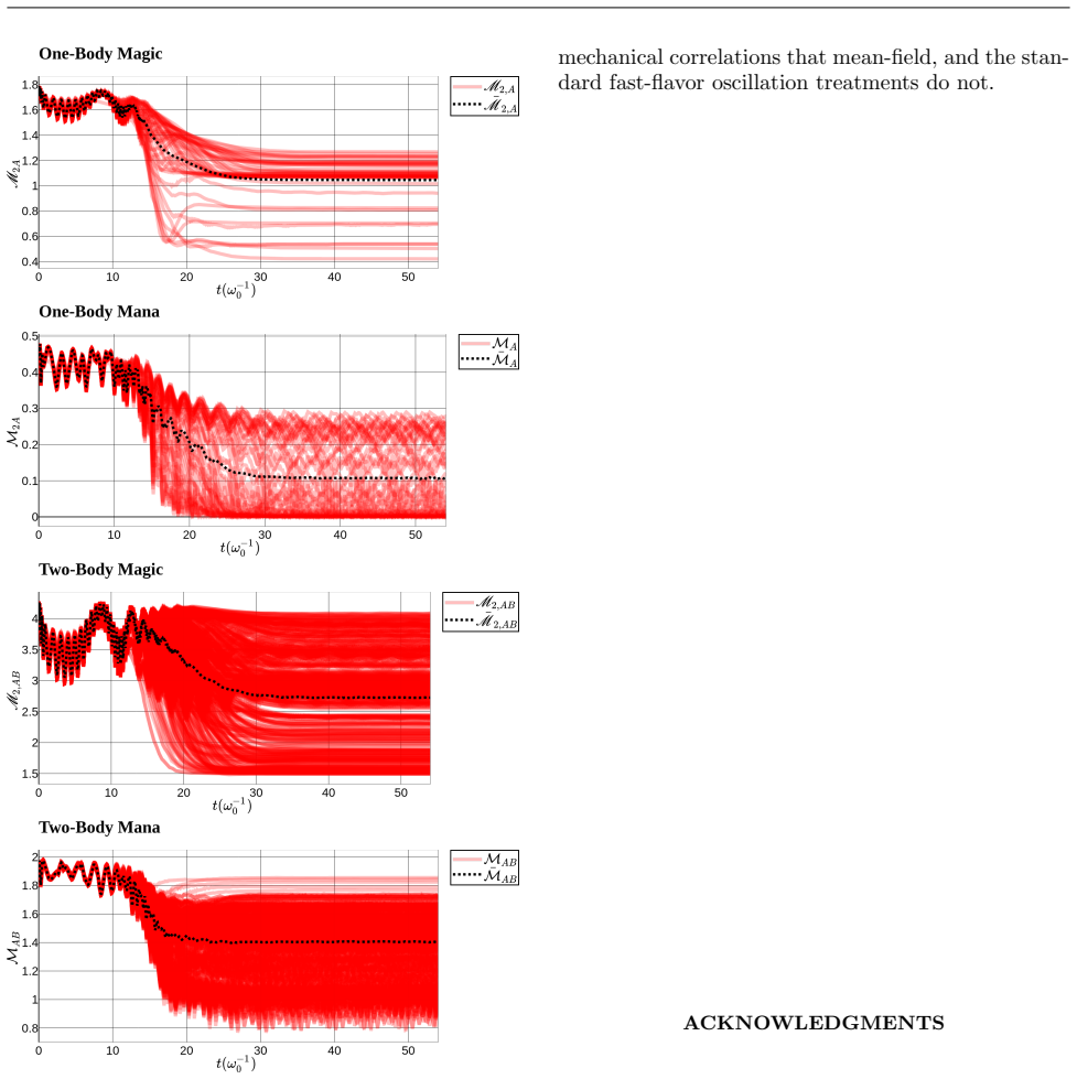
- Mana and magic leak from one-body into higher-body operators across the dynamical crossover, so late-time states need not be classically simulable in the Gottesman–Knill sense.
- The same truncation applies at once to other quadratic su(n) models (Hubbard, Heisenberg, nuclear shell models, etc.).
- Angular averaging by Monte-Carlo sampling of the geometric factors can be combined with the hierarchy equations without spoiling the polynomial scaling.
Where Pith is reading between the lines
- Because the neglected three-body diagrams are O(μ²/N²), the truncation may stay accurate even at realistic supernova densities once the gas dilutes, giving a controlled late-time window into scrambling.
- The observed negativity of tripartite mutual information suggests supernova neutrino gases naturally generate multipartite entanglement that could serve as a benchmark for quantum-simulation platforms.
- Pushing the closure to fourth order would supply a direct numerical convergence test and quantify residual three-body feedback at N=50–100.
Editorial analysis
A structured set of objections, weighed in public.
Referee Report
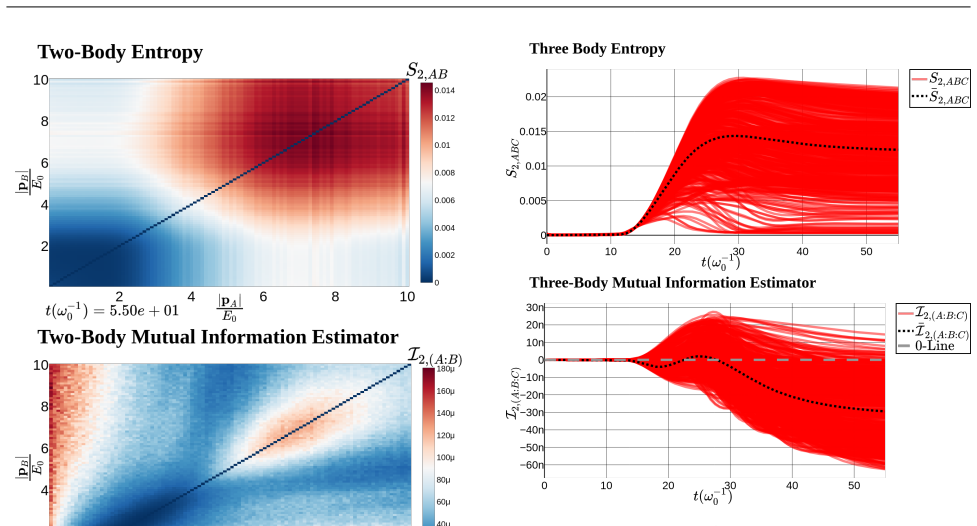
Summary. The manuscript develops a product-algebra formulation of u(n^N) for systems with one- and two-body su(n) Hamiltonians, with collective neutrino oscillations in the forward-scattering limit as the primary application. From this structure it derives compact expressions for multipoint operator expectations, Rényi entropies, Wigner functions, mana, and magic. Dynamics are obtained from the Heisenberg equation, closed by second-order BBGKY truncation (connected three-body cumulants set to zero), yielding coupled ODEs for one- and two-point functions that scale as O(N^3 n^6). For N=4, n=3 the truncated evolution is compared to Trotterized exact dynamics and improves on mean field by roughly two orders of magnitude in Φ and Γ, while reproducing entropy, mana, and magic. The same ODEs are then integrated at N=100 (two flavor) and N=50 (three flavor) with Monte-Carlo angular sampling, and used to report a dynamical crossover near μ(t)∼|B̄|, growth of multipartite Rényi quantities, weak information scrambling, and leakage of non-stabilizer resources into many-body operators.
Significance. If the truncation remains controlled at the N where the physics is extracted, the work supplies a practically useful classical route beyond mean field for all-to-all neutrino Hamiltonians and related quadratic su(n) models, with transparent access to entanglement and non-stabilizerness diagnostics that mean-field and pure phase-space methods do not furnish. The algebraic bookkeeping (product structure, generic Rényi/Wigner formulae, sparse structure-constant contractions) is reusable and clearly presented. The small-system Trotter benchmark is clean and demonstrates a genuine improvement over mean field. Polynomial scaling is a real practical gain relative to exact classical evolution. These strengths make the methodological core worth publishing once the large-N accuracy claim is either better controlled or more carefully delimited.
major comments (3)
- [Sec. III.B, Eq. (52); Sec. V.B–V.D, Figs. 2–4 vs. 6–17] The central physics claims (dynamical crossover, entropy/mutual-information growth, weak scrambling, magic leakage) are drawn from N=50–100 runs of the second-order closure ⟨δΛ_Aa δΛ_Bb δΛ_Cc⟩→0 in Eq. (52). The only quantitative fidelity check against independent dynamics is the single Trotter comparison at N=4, n=3, μ(0)=5 (Figs. 2–4). At that size the Hilbert space is 3^4=81 and the neglected connected diagrams (Eqs. 56–61) are not parametrically small. The text argues those diagrams are O(μ²/N²) and “exceedingly small for N∼10^57,” but does not measure residual truncation error at the N actually simulated (~10^{-3}–10^{-4} suppression). Without a higher-order closure, a small-N convergence series in truncation order, or another independent large-N reference, the accuracy of the large-N entropy/mana/magic interpretations remains uncontrolled. Either supply such a check or reframe Sec.
- [Sec. V.C.1, Fig. 6; Sec. V.D, Fig. 12] The identification of a “dynamical phase transition” (Figs. 6, 12 and surrounding text) rests on a rapid change of the site-averaged order parameter Φ̄_a near μ(t)∼|B̄|. No finite-size scaling, susceptibility peak, or order-parameter distribution is given, and the same qualitative drop appears already in mean field. The language should be tightened to “dynamical crossover” unless a sharper diagnostic is provided, and it should be stated explicitly which features (e.g. two-body cumulant growth, entropy production) are absent in mean field and therefore truncation-dependent.
- [Sec. IV.A, Eqs. (64)–(65)] Positivity and purity bounds (Eqs. 64–65) are enforced by projecting n-point functions onto the nearer bound after each step. This is a nonlinear intervention not implied by the truncated Heisenberg flow. The manuscript should quantify how often and how strongly the projection fires in the N=50–100 runs, and whether entropy, mana, and magic time series change when the projection is disabled or replaced by a softer constraint. Without that, part of the reported late-time behavior could be an artifact of the stabilizer rather than of the BBGKY closure.
minor comments (5)
- [Sec. II.C.1; Figs. 10, 16] The naïve Rényi mutual information I^Naive_α (Eqs. 21, 23) is used extensively; the text correctly notes subadditivity holds only for α=1, but several figure captions still read as if negativity of I_3 is unambiguous evidence of scrambling. A short clarifying sentence in the captions of Figs. 10 and 16 would help.
- [Throughout; References] Typos and notation: “Hierarchy T runcation” / “COMPUT A TIONAL” (Sec. III.B, IV titles); “adoptive” → “adaptive” (Sec. IV.A); “Tructating” → “Truncating” (Sec. V.B); “weather or not” → “whether or not” (Sec. II.C.1); “ban be written” → “can be written” (Sec. II.B). arXiv IDs in the reference list with years 2026 look like placeholders and should be checked.
- [Sec. IV.B, Fig. 1] Fig. 1 caption states second-order truncation scales as O(N^3 n^6); the main text sometimes writes the same and sometimes the binomial form. State one consistent leading-order expression and note the sparse-contraction prefactor actually used.
- [Sec. V.A, V.C–V.D] Monte-Carlo angular integration: number of Π_AB samples (100 for su(2), 50×100 wording for su(3)) and the momentum discretization δ|p| should be stated once in a single “numerical parameters” paragraph so runs are reproducible.
- [Sec. II.C.3, Eq. (40)] Eq. (40) for magic mixes a Pauli-symbol Rényi with S_2; a one-line check that the reported one-body magic vanishes on stabilizer states in the n=2 numerics would reassure readers unfamiliar with the definition.
Circularity Check
No circularity: BBGKY truncation is an explicit ansatz validated against independent Trotter evolution, not a quantity forced by its own inputs.
full rationale
The derivation chain is: (i) product structure of u(n^N) from the su(n) structure constants (Eqs. 11–16); (ii) Heisenberg EOM for n-point operators yielding the BBGKY hierarchy (Eq. 48); (iii) explicit closure by setting the connected three-body cumulant to zero (Eq. 52 and surrounding text); (iv) numerical integration of the closed 1- and 2-body ODEs; (v) comparison to independent Trotter evolution of the same Hamiltonian at N=4, n=3. Nothing in steps (i)–(iv) defines the target observables (Φ, Γ, Rényi entropies, mana, magic) in terms of a fit to those same observables. Mixing angles, Δm², and the bulb-model μ(t) are external inputs. Self-citations (prior Balantekin path-integral/mean-field work, Volpe BBGKY reviews) supply background and motivation but are not used as uniqueness theorems or as the sole justification of the truncation; the truncation is stated as an ansatz and checked against an external benchmark. Large-N physics claims inherit uncontrolled truncation error (a correctness issue), but that is not circularity under the stated criteria. Score 0; steps empty.
Axiom & Free-Parameter Ledger
free parameters (5)
- μ0 (initial interaction strength) =
μ(0)=5 in benchmark and large-N runs
- ω0 (energy unit) =
Δ01/(4E0), E0~10 MeV
- Monte-Carlo angular sample size =
100 (su(2)); 50 angles × 100 samples (su(3))
- δtmax / ε adaptive-step controls
- Momentum magnitude discretization δ|p| and N =
N=4 (benchmark), 100 (su(2)), 50 (su(3))
axioms (5)
- domain assumption Forward-scattering (angle-dependent but momentum-exchange-free) two-body neutrino Hamiltonian of the form H=B·Λ+(μ/2N)Π_AB Λ_A·Λ_B
- ad hoc to paper Three-body connected cumulants vanish identically, closing the BBGKY hierarchy at the two-body level
- standard math su(n) / u(n^N) product algebra and completeness of the generalized Gell-Mann (and clock/Pauli) bases for operator decomposition
- domain assumption Phenomenological neutrino bulb model for μ(t) and vacuum mixing angles/mass splittings taken from global fits
- ad hoc to paper Naïve Rényi mutual information I_α=S_A+S_B−S_AB remains a useful probe even though subadditivity holds only for α=1
read the original abstract
A one- and two-body $\mathfrak{su}(n)$ Hamiltonian governing the dynamics of many systems, including collective neutrino oscillations, is investigated. We start by analyzing the algebraic structure($\mathfrak{u}(n^N)$), formulate a product structure of the algebra, and utilize this to construct generic expressions for operator expectation values, R\'{e}nyi Entropy, and Wigner Functions. Performing BBGKY hierarchy truncation we develop a systematic methodology for going beyond the mean field with polynomial scaling on a classical computer.
Figures




Reference graph
Works this paper leans on
-
[1]
[40]) we can decompose any arbitraryn N ×n N matrix in terms of them: O= 1 nN Tr(O) + 1 nN−1 2 Tr OΛAa ΛAa +
Operator Decomposition, Completeness, Operator Transformations, and Operator Action Since all possible products of Λ AµA ’s are Hermi- tian matrices of the fundamental representation of theu(n N ) algebra (for an explicit illustration see Ref. [40]) we can decompose any arbitraryn N ×n N matrix in terms of them: O= 1 nN Tr(O) + 1 nN−1 2 Tr OΛAa ΛAa +... =...
-
[2]
To examine the entanglement structure, we introduce the R´ enyi En- tropy: Sα,{A} = 1 1−α ln Tr ρα {A} (19) Forα= 1 R´ enyi Entropy reduces to the von Neumann entropy
R´ enyi Entropy & R´ enyi Mutual Information In many-body physics, the entanglement structure is often the primary lens through which we exam- ine the behavior of largeN-systems. To examine the entanglement structure, we introduce the R´ enyi En- tropy: Sα,{A} = 1 1−α ln Tr ρα {A} (19) Forα= 1 R´ enyi Entropy reduces to the von Neumann entropy. Forα= 2, U...
-
[3]
quantum- ness
Discrete Phase Space and Mana Another fundamental characteristic of these many- body systems is their representation in phase space via the Wigner function. The Wigner function provides a quasi probability distribution that maps the many- body density matrix onto a discrete phase space, of- fering a direct visual and mathematical diagnostic of quantum non...
-
[4]
Pauli Symbol
Mana to Magic The Gottesman-Knill theorem states that quantum systems that utilize only stabilizer resources, i.e. cir- cuits that only consist of gates from the Pauli or Clif- ford groups, can be efficiently simulated in polynomial time on a probabilistic classical computer [45]. Thus, it is important to have a measure for the amount of non-stabilizer re...
-
[5]
H. Duan, G. M. Fuller, and Y.-Z. Qian, Ann. Rev. Nucl. Part. Sci.60, 569 (2010), arXiv:1001.2799 [hep- ph]
Pith/arXiv arXiv 2010
-
[6]
A. B. Balantekin, J. Phys. G45, 113001 (2018), arXiv:1809.02539 [hep-ph]
Pith/arXiv arXiv 2018
-
[7]
I. Tamborra and S. Shalgar, Ann. Rev. Nucl. Part. Sci.71, 165 (2021), arXiv:2011.01948 [astro-ph.HE]
Pith/arXiv arXiv 2021
-
[8]
L. Johns, S. Richers, and M.-R. Wu, Ann. Rev. Nucl. Part. Sci.75, 399 (2025), arXiv:2503.05959 [astro- ph.HE]
Pith/arXiv arXiv 2025
-
[9]
M. C. Volpe, Rev. Mod. Phys.96, 025004 (2024), arXiv:2301.11814 [hep-ph]
Pith/arXiv arXiv 2024
-
[10]
A. B. Balantekin and Y. Pehlivan, J. Phys. G34, 47 (2007), arXiv:astro-ph/0607527
Pith/arXiv arXiv 2007
-
[11]
M. J. Cervia, A. V. Patwardhan, A. B. Balantekin, ‡. S. N. Coppersmith, and C. W. Johnson, Phys. Rev. D100, 083001 (2019), arXiv:1908.03511 [hep-ph]
Pith/arXiv arXiv 2019
-
[12]
M. J. Cervia, P. Siwach, A. V. Patwardhan, A. B. Balantekin, S. N. Coppersmith, and C. W. Johnson, Phys. Rev. D105, 123025 (2022), arXiv:2202.01865 [hep-ph]
Pith/arXiv arXiv 2022
-
[13]
D. Lacroix, A. B. Balantekin, M. J. Cervia, A. V. Pat- wardhan, and P. Siwach, Phys. Rev. D106, 123006 (2022), arXiv:2205.09384 [nucl-th]. 16
Pith/arXiv arXiv 2022
-
[14]
M. Illa and M. J. Savage, Phys. Rev. Lett.130, 221003 (2023), arXiv:2210.08656 [nucl-th]
Pith/arXiv arXiv 2023
-
[15]
J. D. Martin, A. Roggero, H. Duan, J. Carlson, and V. Cirigliano, Phys. Rev. D105, 083020 (2022), arXiv:2112.12686 [hep-ph]
Pith/arXiv arXiv 2022
-
[16]
J. D. Martin, D. Neill, A. Roggero, H. Duan, and J. Carlson, Phys. Rev. D108, 123010 (2023), arXiv:2307.16793 [hep-ph]
Pith/arXiv arXiv 2023
- [17]
-
[18]
D. Lacroix, A. Bauge, B. Yilmaz, M. Mangin-Brinet, A. Roggero, and A. B. Balantekin, Phys. Rev. D110, 103027 (2024), arXiv:2409.20215 [hep-ph]
Pith/arXiv arXiv 2024
-
[19]
D. Neill, H. Liu, J. Martin, and A. Roggero, Phys. Rev. Res.7, 023157 (2025), arXiv:2406.18677 [hep- ph]
Pith/arXiv arXiv 2025
-
[20]
I. Chernyshev, C. E. P. Robin, and M. J. Savage, Phys. Rev. Res.7, 023228 (2025), arXiv:2411.04203 [quant-ph]
Pith/arXiv arXiv 2025
-
[21]
Bhaskar, A
R. Bhaskar, A. Roggero, and M. J. Savage, Phys. Rev. C110, 045801 (2024)
2024
-
[22]
F. Br¨ okemeier, S. M. Hengstenberg, J. W. T. Keeble, C. E. P. Robin, F. Rocco, and M. J. Savage, Phys. Rev. C111, 034317 (2025), arXiv:2409.12064 [nucl- th]
Pith/arXiv arXiv 2025
-
[23]
O. Kiss, I. Tavernelli, F. Tacchino, D. Lacroix, and A. Roggero, (2025), arXiv:2510.24841 [quant-ph]
arXiv 2025
-
[24]
Z. Laraib and S. Richers, Phys. Rev. D112, L101304 (2025), arXiv:2507.02040 [astro-ph.HE]
Pith/arXiv arXiv 2025
-
[25]
Z. Laraib and S. Richers, Phys. Rev. D112, 123045 (2025), arXiv:2511.16506 [astro-ph.HE]
Pith/arXiv arXiv 2025
- [26]
-
[27]
J. Froustey, E. Rrapaj, Y. Liu, G. Li, C. Iancu, and V. Cirigliano, (2026), arXiv:2606.12404 [hep-ph]
Pith/arXiv arXiv 2026
-
[28]
K. Yeter-Aydeniz, S. Bangar, G. Siopsis, and R. C. Pooser, Quant. Inf. Proc.21, 84 (2022), arXiv:2104.03273 [quant-ph]
Pith/arXiv arXiv 2022
-
[29]
V. Amitrano, A. Roggero, P. Luchi, F. Turro, L. Vespucci, and F. Pederiva, Phys. Rev. D107, 023007 (2023), arXiv:2207.03189 [quant-ph]
Pith/arXiv arXiv 2023
-
[30]
B. Hall, A. Roggero, A. Baroni, and J. Carlson, Phys. Rev. D104, 063009 (2021), arXiv:2102.12556 [quant- ph]
Pith/arXiv arXiv 2021
-
[31]
P. Siwach, K. Harrison, and A. B. Balantekin, Phys. Rev. D108, 083039 (2023), arXiv:2308.09123 [quant- ph]
Pith/arXiv arXiv 2023
-
[32]
A. B. Balantekin, M. J. Cervia, A. V. Patwardhan, E. Rrapaj, and P. Siwach, Eur. Phys. J. A59, 186 (2023), arXiv:2305.01150 [nucl-th]
Pith/arXiv arXiv 2023
-
[33]
F. Turro, I. A. Chernyshev, R. Bhaskar, and M. Illa, Phys. Rev. D111, 043038 (2025), arXiv:2407.13914 [quant-ph]
Pith/arXiv arXiv 2025
-
[34]
L. Spagnoliet al., Phys. Rev. D111, 103054 (2025), arXiv:2503.00607 [quant-ph]
Pith/arXiv arXiv 2025
-
[35]
D. J. Heimsoth, A. B. Balantekin, and P. Siwach, Three-flavor supernova neutrino simulation using a hybrid quantum-classical algorithm with qutrits (2026), arXiv:2605.01099 [hep-ph]
Pith/arXiv arXiv 2026
-
[36]
A. Roggero, Phys. Rev. D104, 103016 (2021), arXiv:2102.10188 [hep-ph]
Pith/arXiv arXiv 2021
-
[37]
M. Mangin-Brinet, A. Bauge, and D. Lacroix, Phys. Rev. D113, 036026 (2026), arXiv:2507.18482 [hep- ph]
Pith/arXiv arXiv 2026
-
[38]
C. Volpe, D. V¨ a¨ an¨ anen, and C. Espinoza, Phys. Rev. D87, 113010 (2013), arXiv:1302.2374 [hep-ph]
Pith/arXiv arXiv 2013
-
[39]
D. V¨ a¨ an¨ anen and C. Volpe, Phys. Rev. D88, 065003 (2013), arXiv:1306.6372 [hep-ph]
Pith/arXiv arXiv 2013
-
[40]
J. Serreau and C. Volpe, Phys. Rev. D90, 125040 (2014), arXiv:1409.3591 [hep-ph]
Pith/arXiv arXiv 2014
-
[41]
D. Bossion and P. Huo, General formulas of the structure constants in thesu(n) lie algebra (2021), arXiv:2108.07219 [math-ph]
Pith/arXiv arXiv 2021
-
[42]
V. Rosenhaus, J. Phys. A52, 323001 (2019), arXiv:1807.03334 [hep-th]
Pith/arXiv arXiv 2019
-
[43]
Kitaev, Annals Phys.321, 2 (2006), arXiv:cond- mat/0506438
A. Kitaev, Annals Phys.321, 2 (2006), arXiv:cond- mat/0506438
arXiv 2006
-
[44]
A. B. Balantekin and A. M. Suliga, Eur. Phys. J. A 60, 124 (2024), arXiv:2405.13862 [quant-ph]
Pith/arXiv arXiv 2024
-
[45]
´A. M. Alhambra, PRX Quantum4, 040201 (2023), arXiv:2204.08349 [quant-ph]
Pith/arXiv arXiv 2023
-
[46]
S. O. Scalet, ´A. M. Alhambra, G. Styliaris, and J. I. Cirac, Quantum5, 541 (2021), arXiv:2103.01709 [quant-ph]
Pith/arXiv arXiv 2021
-
[47]
A. Seshadri, V. Madhok, and A. Lakshminarayan, Phys. Rev. E98, 052205 (2018), arXiv:1806.00113 [quant-ph]
Pith/arXiv arXiv 2018
-
[48]
G. Bjrk, A. B. Klimov, and L. L. Snchez-Soto (Else- vier, 2008) pp. 469–516
2008
-
[49]
Gottesman, in22nd International Colloquium on Group Theoretical Methods in Physics(1998) pp
D. Gottesman, in22nd International Colloquium on Group Theoretical Methods in Physics(1998) pp. 32– 43, arXiv:quant-ph/9807006
Pith/arXiv arXiv 1998
-
[50]
L. Leone, S. F. E. Oliviero, and A. Hamma, Phys. Rev. Lett.128, 050402 (2022), arXiv:2106.12587 [quant-ph]
Pith/arXiv arXiv 2022
-
[51]
Salasnich and C
L. Salasnich and C. Vianello, SciPost Phys. Lect. Notes117, 1 (2026)
2026
-
[52]
R. Kubo, J. Phys. Soc. Jap.17, 1100 (1962)
1962
-
[53]
M. E. Peskin and D. V. Schroeder,An Introduction to quantum field theory(Addison-Wesley, Reading, USA, 1995)
1995
-
[54]
V. Cirigliano, S. Sen, and Y. Yamauchi, Phys. Rev. D 110, 123028 (2024), arXiv:2404.16690 [hep-ph]
Pith/arXiv arXiv 2024
-
[55]
M. J. Cervia, Phys. Rev. D113, 043010 (2026), arXiv:2510.22005 [hep-ph]
arXiv 2026
-
[56]
Kuehn, Moment closure—a brief review, inCon- trol of Self-Organizing Nonlinear Systems, edited by E
C. Kuehn, Moment closure—a brief review, inCon- trol of Self-Organizing Nonlinear Systems, edited by E. Sch¨ oll, S. H. L. Klapp, and P. H¨ ovel (Springer In- ternational Publishing, Cham, 2016) pp. 253–271
2016
-
[57]
H. Duan, G. M. Fuller, J. Carlson, and Y.-Z. Qian, Phys. Rev. D74, 105014 (2006), arXiv:astro- ph/0606616
arXiv 2006
-
[58]
Hilfer, B
R. Hilfer, B. Biswal, H.-G. Mattutis, and W. Janke, Computer Physics Communications169, 230 (2005), proceedings of the Europhysics Conference on Com- putational Physics 2004
2005
-
[59]
J. J. Wallman and S. D. Bartlett, Phys. Rev. A85, 062121 (2012), arXiv:1203.2652 [quant-ph]
Pith/arXiv arXiv 2012
-
[60]
R. J. Garcia, K. Bu, and A. Jaffe, Proc. Nat. Acad. Sci.120, e2217031120 (2023), arXiv:2208.10477 [quant-ph]. 17
Pith/arXiv arXiv 2023
discussion (0)
Sign in with ORCID, Apple, or X to comment. Anyone can read and Pith papers without signing in.