REVIEW 4 major objections 4 minor 28 references
A differentiable loss function makes thermodynamic model fitting a direct gradient-descent problem.
Reviewed by Pith at T0; open to challenge. T0 means a machine referee read the full paper against a public rubric. the ladder, T0–T4 →
T0 review · deepseek-v4-flash
2026-08-05 00:46 UTC pith:ZM3VJAEJ
load-bearing objection A genuinely useful auto-diff phase-equilibrium loss with a real gap between the exact theory and the approximate numerics; worth peer review but the sufficient-and-necessary claim needs softening or support. the 4 major comments →
Machine Learning Compatible CALPHAD-type Optimization from Phase Equilibria by Auto-differentiation
The pith
A machine-rendered reading of the paper's core claim, the machinery that carries it, and where it could break.
Core claim
The central discovery is that the equilibrium condition for stable phases can be turned into a differentiable loss: for each observed phase, evaluate the Gibbs energy at the observed composition minus the auxiliary chemical-potential dot product, plus the minimized grand potential at that auxiliary potential; for each phase that should be absent, add a ReLU penalty on the negative minimized grand potential. When the auxiliary chemical potentials are optimized alongside the model parameters, this loss reaches zero if and only if the observed phase equilibrium is reproduced. Because the loss is defined from equilibrium conditions rather than from a particular free-energy expression, it applies
What carries the argument
The loss is L = sum over stable phases of |G_m(X,W) - mu'·X|^p + |min_y Phi_m(y,mu',W)|^p + sum over absent phases of ReLU(-min_y Phi_m(y,mu',W)), where Phi = G - mu'·N is the grand potential at an auxiliary chemical potential mu' that is itself an optimization variable. Exponential gradient descent on the simplex, with linear composition constraints handled by Newton-solved multipliers, locates the internal-coordinate minima; the envelope theorem detaches those minimizers from the gradient graph; and a Softmin with tau = 1/log(n) approximates the minimum with a claimed sub-1 J/mol error.
Load-bearing premise
The optimization assumes the random grid plus finite exponential-gradient-descent steps finds the true global minimum of the Gibbs and grand-potential functions over internal coordinates; if the free-energy surface is non-convex or the grid is too sparse, the loss and its gradients become biased even though the loss can still be small.
What would settle it
Take a binary system whose free-energy surfaces are known to have a deep metastable minimum, generate a target two-phase equilibrium, and run the optimizer with a coarse grid versus a very dense grid. If the coarse-grid run drives the loss to near zero but an independent global-equilibrium calculation shows the optimized model does not actually reproduce the observed phase compositions, the sufficiency claim fails.
If this is right
- Model parameters of any differentiable thermodynamic model can be optimized directly against experimental phase-equilibrium data without a separate global equilibrium calculation at each step.
- Because no global equilibrium solve is needed, the optimizer scales to ternary CALPHAD assessments with more than one hundred parameters, as shown in the Al–Mo–Si example.
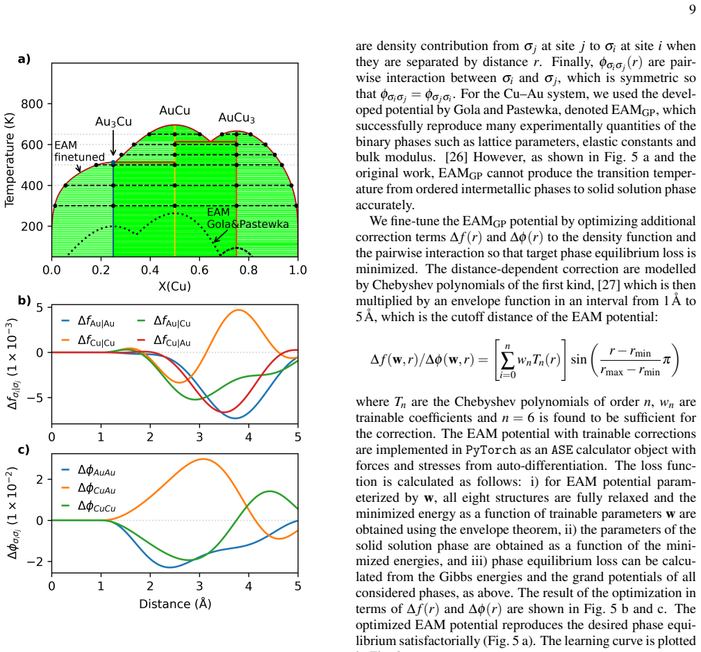
- The same loss can fine-tune an atomistic potential, so a single parameterization can simultaneously reproduce target phase transitions and remain usable for other downstream calculations such as Monte Carlo ordering simulations.
- When a phase equilibrium is exactly reproduced, the loss reaches zero, giving a clear stopping criterion; the auxiliary chemical potential construction also handles cases where only one side of a two-phase equilibrium has a measured composition.
Where Pith is reading between the lines
- Because the loss does not require knowing which phase is the global minimum, it could be used to co-calibrate multiple models against conflicting or uncertain phase-boundary data with weights, though the paper does not demonstrate uncertainty weighting.
- The inner-minimization accuracy is the main thing to test: in non-convex energy landscapes, one would inspect whether the same optimized parameters survive when the random grid is replaced by a much denser one, or by a different global optimizer.
- The top-down atomistic-potential result suggests a route to correct machine-learned interatomic potentials using only experimental transition temperatures, without needing to retain the original DFT reference energies; this would need tests on systems with vibrational entropy included.
- The Softmin approximation error is claimed below 1 J/mol at tau = 1/log(n); a direct numerical check on a pathological multi-well model would tell whether that bound holds at finite n.
Editorial analysis
A structured set of objections, weighed in public.
Referee Report
Summary. The paper proposes a differentiable loss function for optimizing thermodynamic model parameters directly from phase-equilibrium data, avoiding explicit global equilibrium calculations. The loss is derived from the stationarity conditions of the global equilibrium problem: for each observed stable phase, it penalizes the distance of the composition-constrained Gibbs energy to an auxiliary chemical-potential hyperplane and the minimum of the corresponding grand potential, while unobserved phases contribute a ReLU penalty on negative grand-potential minima. The auxiliary chemical potentials are either eliminated when the number of phases equals the number of components or optimized jointly with the model parameters. Inner minimizations over internal coordinates are performed by random sampling (Dirichlet and hit-and-run), a finite number of exponential-gradient-descent (EGD) steps, and a Softmin aggregation, all implemented in PyTorch for auto-differentiation. The method is demonstrated on Al–Zn, Cu–Mg, and Al–Mo–Si CALPHAD models and on fine-tuning an EAM potential for Au–Cu.
Significance. If the numerical inner minimizations are reliable, the contribution is significant and timely. The loss function provides a model-agnostic, differentiable objective for CALPHAD and machine-learning thermodynamic models, and the EAM fine-tuning example demonstrates a genuinely new capability. The derivation from equilibrium conditions is conceptually clean, and the availability of code is a practical strength. The main risk is that the formal zero-loss equivalence is stated as exact while the implementation relies on approximate inner minimization with unquantified gaps; this is the load-bearing issue for the paper's central claim.
major comments (4)
- [Section II.B and II.D] The statement 'As the loss function is derived from equilibrium condition, its value equal to zero is a sufficient and necessary condition for observed phase equilibrium to be reproduced' is exact only when the inner minimizations min_y G and min_y Phi are exact. In Section II.D these are replaced by a random grid plus a finite number of EGD steps plus Softmin. The text asserts that 'a relatively dense sample grid, small number of gradient descent step is sufficient to ensure that a global minimium can be found', but no guarantee or verification is provided. CEF and EAM free-energy surfaces are generally non-convex, and EGD is a local method. The paper should either supply a convergence guarantee or, minimally, verify for representative cases (e.g., by comparison with a global optimizer and by reporting grid size and number of EGD steps) that the approximate minima are close to the true
- [Section II.D] The claimed Softmin error bound of '<1 J/mol by setting τ=1/log(n)' is not derived or referenced. As written, Softmin only controls the smoothing bias relative to the best sampled point; it does not bound the gap between the best sampled point and the true global minimum. The error also depends on the energy range of the samples. This claim is load-bearing for the accuracy of the loss and its gradients and should be either proved with explicit assumptions or replaced by a more defensible error-control mechanism.
- [Appendix A and Section II.B] The envelope theorem is invoked to detach the minimizing internal coordinates y* from the auto-differentiation graph. The theorem requires x*(ω) to be a true minimizer. For the approximate y* returned by grid+EGD+Softmin, ∂y*/∂W is nonzero and is neglected, so the computed loss gradient is biased. The magnitude of this bias is not quantified. To support the optimization results, the authors should compare the detached-gradient approach with a direct differentiation through the inner minimization, or otherwise demonstrate that the bias is negligible near the reported optima.
- [Section III] All demonstrations train on the full set of phase-equilibrium data and judge success by training error and visual agreement with phase diagrams. The text explicitly states: 'we have used all input data for training for simplification'. This is a stated limitation, but it is load-bearing for the claim that the method 'successfully optimizes' thermodynamic models. The paper should report final training loss values and, for at least one binary and the ternary system, evaluate on held-out phase-equilibrium data or quantify phase-boundary errors against the reference assessments. Otherwise the demonstrations are self-consistency checks rather than evidence of predictive optimization.
minor comments (4)
- [Introduction] Typo: 'revelant phases diagrams' should be 'relevant phase diagrams'. Also, 'CALPHAD' is capitalized inconsistently (e.g., 'Calphad' in several places).
- [Section II.B] The phrase 'we should, in addition, compute the same time at the constrained composition' should read 'at the same time'. Also, the notation for the loss function would benefit from explicitly labeling the terms, since the current display is dense.
- [Section III] The code availability statement contains the placeholder '[url]' rather than a concrete DOI or repository URL. This should be completed before publication.
- [Figure 3] The caption text describes the examples as Al–Zn, Cu–Mg, and Al–Mo–Si, but the figure also includes Cu–Au. Please update the caption to mention all four systems.
Circularity Check
No circularity: the loss is a fitting objective derived from equilibrium conditions; no prediction is claimed and no load-bearing self-citation.
full rationale
The paper's central derivation (Sec. II.A-II.B) constructs a loss function L(mu',W) from the equilibrium condition: for each observed stable phase, the difference between the composition-constrained Gibbs energy and the tangent plane at auxiliary chemical potential mu', plus the unconstrained grand-potential minimum, and for unobserved phases a ReLU penalty on the grand-potential minimum. Zero of this loss is shown equivalent to existence of a common mu' for which every observed composition minimizes the grand potential and no unobserved phase has negative grand potential; this is exactly the common-tangent equilibrium condition. This is a fitting objective, not a prediction: Section III explicitly states all input data are used for training and success is judged on training error and the resulting phase diagrams. There is no fitted parameter disguised as a prediction, and no held-out prediction is claimed. The references to prior work by the authors (e.g., NIMS CPDDB [18], used only as the source of target assessments for the demonstration) are not load-bearing for the derivation; the loss derivation is self-contained. The Softmin/grid+EGD approximation in Sec. II.D and the envelope-theorem treatment in Appendix A are approximations whose accuracy is not proved, but this is a numerical-correctness risk, not circularity. Therefore no circular step is present.
Axiom & Free-Parameter Ledger
free parameters (5)
- regularization weight λ =
not reported
- Softmin temperature τ =
1/log(n)
- EGD step size and number of steps =
not reported
- Chebyshev order n =
6
- number of grid samples =
not reported
axioms (4)
- domain assumption Global equilibrium is obtained by minimizing total Gibbs energy under mass-balance and non-negativity constraints
- domain assumption The CEF and EAM free-energy expressions are differentiable in the parameters W and internal coordinates y
- ad hoc to paper The inner minimization problems over y have a unique global minimum and the solution is an interior point so the envelope theorem applies
- ad hoc to paper Softmin with τ=1/log(n) approximates the true minimum within 1 J/mol
Cite this review
Pith. "Pith review of Machine Learning Compatible CALPHAD-type Optimization from Phase Equilibria by Auto-differentiation." pith.science (2026). https://pith.science/paper/ZM3VJAEJ
@misc{pith2026260800516,
  author       = {Pith},
  title        = {Pith review of: Machine Learning Compatible CALPHAD-type Optimization from Phase Equilibria by Auto-differentiation},
  year         = {2026},
  howpublished = {\url{https://pith.science/paper/ZM3VJAEJ}},
  note         = {Machine review of arXiv:2608.00516}
}
read the original abstract
To accurately determine phase boundaries and phase transitions, thermodynamic models that describe free energies of phases often have to be optimized based on experimentally observed phase equilibria. While different approaches exist for thermodynamic optimizations, these approaches are often implemented in ways that are not compatible with machine learning workflows that requires differentiable calculation of loss function. In this work, we derive a phase equilibrium loss function based on thermodynamic potentials that can be efficiently evaluated and enable gradient based optimization by auto-differentiation in the PyTorch package. By minimizing this loss function, general thermodynamic model parameters can be optimized with respect to experimental phase equilibria data. Using thermodynamic models in the CALculation of PHAse Diagram (CALPHAD) framework, We illustrate successful and efficient optimization in different systems including ternary ones with more than 100 parameters. As the loss function is defined independently of the details of the thermodynamic models, it can be used to optimize machine learning thermodynamic models in general. In particular, we demonstrate a top-down optimization of atomistic potential from target phase equilibria.
Figures


Reference graph
Works this paper leans on
- [1]
-
[2]
Z.-K. Liu, Thermodynamics and its prediction and CALPHAD modeling: Review, state of the art, and perspectives, Calphad 82, 102580 (2023)
work page 2023
-
[3]
A. Togo and I. Tanaka, First principles phonon calculations in materials science, Scripta Materialia108, 1 (2015)
work page 2015
-
[4]
A. V . D. Walle and M. Asta, Self-driven lattice-model Monte Carlo simulations of alloy thermodynamic properties and phase diagrams, Modelling Simul. Mater. Sci. Eng.10, 521 (2002)
work page 2002
-
[5]
J. Riebesell, R. E. A. Goodall, P. Benner, Y . Chiang, B. Deng, G. Ceder, M. Asta, A. A. Lee, A. Jain, and K. A. Persson, A framework to evaluate machine learning crystal stability pre- dictions, Nat Mach Intell7, 836 (2025)
work page 2025
-
[6]
M. Poul, L. Huber, and J. Neugebauer, Automated generation of structure datasets for machine learning potentials and alloys, npj Comput Mater11, 174 (2025)
work page 2025
-
[7]
S. Zhu, D. Sarıtürk, and R. Arróyave, Accelerating CALPHAD- based phase diagram predictions in complex alloys using uni- versal machine learning potentials: Opportunities and chal- lenges, Acta Materialia286, 120747 (2025)
work page 2025
-
[8]
C. Kunselman, B. Bocklund, A. Van De Walle, R. Otis, and R. Arróyave, Analytically differentiable metrics for phase sta- bility, Calphad86, 102705 (2024)
work page 2024
-
[9]
C. Kunselman, B. Bocklund, R. Otis, and R. Arroyave, Analyti- cal Gradient-Based Optimization of CALPHAD Model Param- eters (2025)
work page 2025
-
[10]
Guan, Differentiable thermodynamic modeling, Scripta Materialia207, 114217 (2022)
P.-W. Guan, Differentiable thermodynamic modeling, Scripta Materialia207, 114217 (2022)
work page 2022
- [11]
-
[12]
F. Tang and B. Hallstedt, Using the PARROT module of Thermo-Calc with the Cr–Ni system as example, Calphad55, 260 (2016)
work page 2016
-
[13]
B. Reis, F. Tang, P. Keuter, and M. to Baben, User-friendly and robust Calphad optimizations using Calphad Optimizer in Fact- Sage, Calphad88, 102800 (2025)
work page 2025
-
[14]
B. Sundman, X.-G. Lu, and H. Ohtani, The implementation of an algorithm to calculate thermodynamic equilibria for multi- component systems with non-ideal phases in a free software, Computational Materials Science101, 127 (2015)
work page 2015
-
[15]
B. Bocklund, R. Otis, A. Egorov, A. Obaied, I. Roslyakova, and Z.-K. Liu, ESPEI for efficient thermodynamic database devel- opment, modification, and uncertainty quantification: Applica- tion to Cu–Mg, MRS Communications9, 618 (2019)
work page 2019
-
[16]
We have defined a quantityΦ, which has the form of a grand potential (since it is a function of the chemical poten- tial): Φα M(yα ,µ,W α ) =Gα M(yα ,W α )− ∑ A µANα A (yα ) The stationary point is given by the following set of equations: ∂L ∂N α =Φ α M(yα ,µ,W α ) ( =0 ifN α >0 >0 ifN α =0 ∂L ∂y α i =N α ∂Φ α M ∂y α i +∑ k ζk Cα k (yα ) ∂y i =0 ∂L ∂ µA =...
-
[17]
M. Hillert, Some viewpoints on the use of a computer for cal- culating phase diagrams, Physica B+C103, 31 (1981)
work page 1981
-
[18]
Kikuchi, Ternary phase diagram calculations—I General the- ory, Acta Metallurgica25, 195 (1977)
R. Kikuchi, Ternary phase diagram calculations—I General the- ory, Acta Metallurgica25, 195 (1977)
work page 1977
-
[19]
T. Abe, K. Hashimoto, Y . Goto, Y . Sawada, and K. Hirose, CPDDB (2007)
work page 2007
-
[20]
R. Otis and Z.-K. Liu, Pycalphad: CALPHAD-based Compu- tational Thermodynamics in Python, JORS5, 1 (2017)
work page 2017
-
[21]
X. Fu, B. M. Wood, L. Barroso-Luque, D. S. Levine, M. Gao, M. Dzamba, and C. L. Zitnick, Learning Smooth and Expres- sive Interatomic Potentials for Physical Property Prediction (2025), arXiv:2502.12147 [physics]
Pith/arXiv arXiv 2025
-
[22]
S. A. Mey, Reevaluation of the Al-Zn System, International Journal of Materials Research84, 451 (1993)
work page 1993
- [23]
-
[24]
Y . Liu, G. Shao, and P. Tsakiropoulos, Thermodynamic re- assessment of the Mo–Si and Al–Mo–Si systems, Intermetallics 8, 953 (2000)
work page 2000
-
[25]
B. Sundman, S. G. Fries, and W. Oates, A thermodynamic as- sessment of the Au-Cu system, Calphad22, 335 (1998)
work page 1998
-
[26]
W. Cao, Y . Chang, J. Zhu, S. Chen, and W. Oates, Thermody- namic modeling of the Cu–Ag–Au system using the cluster/site approximation, Intermetallics15, 1438 (2007)
work page 2007
-
[27]
A. Gola and L. Pastewka, Embedded atom method potential for studying mechanical properties of binary Cu–Au alloys, Mod- elling Simul. Mater. Sci. Eng.26, 055006 (2018)
work page 2018
-
[28]
R. L. Burden and J. D. Faires,Numerical Analysis, 9th ed. (Brooks/Cole, Cengage Learning, Boston, MA, 2011)
work page 2011
discussion (0)
Sign in with ORCID, Apple, or X to comment. Anyone can read and Pith papers without signing in.