Temporal Channel Estimation for Generalized CSI Feedback

Hyeonsu Lyu; Hyun Jong Yang; Minwoo Kim; Sehyun Ryu; Sojeong Park

REVIEW 4 major objections 5 minor 44 references

Temporal Channel Estimation for Generalized CSI Feedback

T0 review · 4 major / 5 minor · reviewed 2026-08-04 · deepseek-v4-flash

Challenge this review Re-run · record.json Download PDF Read on arXiv ↗

Pith's one-line read One neural pass predicts multipath delays, making CSI feedback fast, tiny, and environment-agnostic

desk verdict A well-motivated one-shot neural-CS hybrid with correct local math, but the empirical case, especially cross-domain zero-shot generalization, is internally inconsistent and needs a major revision before the headline numbers can be trusted. read the letter →

arxiv 2608.01713 v1 pith:N3MEUAJO submitted 2026-08-03 eess.SP

Minwoo Kim , Hyeonsu Lyu , Sehyun Ryu , Sojeong Park , Hyun Jong Yang This is my paper · ORCID

classification eess.SP

keywords CSIfeedbackmassiveMIMOcompressedsensingdeeplearningdelay-domainsparsityzero-shotgeneralizationchannelestimationFDDsystems

verification ladder T0 review T1 audit T2 compute T3 formal

The pith

A machine-rendered reading of the paper's core claim, the machinery that carries it, and where it could break.

The reading

TAP claims that one lightweight architecture can satisfy the four practical requirements for FDD massive MIMO CSI feedback: sub-millisecond inference, sub-megabyte model, high reconstruction fidelity, and zero-shot generalization to unseen environments and antenna geometries. It does so by replacing the iterative atom search of compressed sensing with a one-shot 1D convolutional network that predicts continuous multipath delays from a temporal window of channel snapshots, then recovers spatial amplitudes with one closed-form least-squares solve. The base station reconstructs the channel via an inverse Fourier dictionary multiply, needing no neural decoder. If right, the framework lets a single trained model be deployed across different arrays and environments while staying within UE memory and latency budgets.

What carries the argument

The pipeline combines DelayNet, a differentiable sub-grid extractor, a shared continuous Fourier dictionary, and one regularized least-squares solve. DelayNet takes a Hamming-windowed delay-domain temporal sequence, averages across antennas, and uses depthwise separable convolutions so the parameter count is independent of array dimensions; its sigmoid output is a delay heatmap. Parabolic interpolation around the top-K peaks yields continuous delays tau_k. The dictionary A[n,k]=exp(-j2*pi*f_n*tau_k) is built once, the least-squares solve gives the per-antenna amplitudes, and the BS reconstructs the full CFR as H_hat = A X_hat, an inverse-Fourier-style matrix multiply with no neural decoder.

What would settle it

Measure TAP's CFR-NMSE on a spherical-wavefront near-field channel where the same multipath cluster arrives at different antennas with delays differing by more than a small fraction of the sampling interval; if, as Eq. (34) predicts, the error diverges linearly toward the band edges and exceeds a standard far-field baseline, the joint-spatial-sparsity premise is the binding constraint. A second check: train on one environment and test on a completely new ray-traced or measured environment outside the five simulation datasets, and see whether the reported cross-geometry and zero-shot cross-doma

Watch

Extended reading notes

Core claim

The paper's central claim is that the hard part of sparse CSI recovery—finding the continuous delays that carry channel energy—can be learned as a single forward pass of a spatial-agnostic 1D CNN, leaving one least-squares projection to compute per-antenna amplitudes. A differentiable parabolic sub-grid extractor outputs fractional delays, eliminating grid mismatch. Because delays are assumed shared across all antennas, the same Fourier dictionary serves every antenna, the model parameters never depend on array size, and the BS reconstructs the full CFR with no neural decoder. Evaluations across five 3GPP-style environments report 3.13-12.22 dB CFR-NMSE gains over CsiNet variants, under 1 MB

Load-bearing premise

Every antenna sees the same set of physical multipath delays, with differences between antennas appearing only as constant phase shifts in the complex amplitudes; if true delays vary across antennas (near-field wavefronts), the single shared delay estimate and one least-squares solve cannot correct the resulting frequency-dependent phase error.

Editorial extensions

If this is right

A single frozen model transfers to array geometries from 1x32 ULA to 8x8 or 16x4 UPA with less than 3 dB CFR-NMSE penalty.
A model trained on one environment, such as an indoor factory, reconstructs channels in unseen outdoor environments without fine-tuning.
The uplink payload carries only K delays and K x N_ant amplitudes, so the base station needs no neural network; reconstruction is one Fourier dictionary multiply.
The approach meets the 5G NR sub-millisecond latency budget on UE-class hardware, with model size below 1 MB and 0.03-0.15 GFLOPs per inference.
Reporting full CFR-NMSE rather than truncated patch NMSE reveals that DL baselines' real errors are much larger than the values in prior literature, changing how fairness should be evaluated.

Reading between the lines

Editorial extensions of the paper, not claims the author makes directly.

The reported 6 dB-per-bit quantization behavior follows directly from TAP's very low error floor; that suggests rate-adaptive quantization and amplitude compression are natural next steps, since the payload becomes noise-limited by the number of bits per amplitude rather than by model error.
Because the temporal history is identified as a primary denoiser (the W=1 CDL-A case degrades faster under CSI-RS noise), deployment on static or single-snapshot links will rely more on array averaging; a fair test would evaluate TAP with W=1 across all environments.
The same physical principle—shared delays, per-antenna amplitudes—extends to near-field XL-MIMO only if per-antenna delay offsets are added to the dictionary or the model predicts delay spreads; the paper's Eq. (34) gives a concrete error model to test against.
If zero-shot transfer holds on real over-the-air channels, the practical implication is that one universal uplink payload format and one trained model could serve many base station form factors, a deployment simplification beyond the simulations reported here.

Share X Bluesky LinkedIn Reddit HN

Editorial analysis

A structured set of objections, weighed in public.

Desk editor's note, referee report, and a circularity audit.

Desk Editor's Note

read the letter

TAP is a genuinely promising hybrid: a one-shot CNN delay estimator, differentiable sub-grid extraction, and a single least-squares solve with a decoder-free BS. If the numbers hold, it is a real step for FDD massive MIMO. The local theory is solid: the error bound in Section IV-B is a standard projector argument and it works, and the near-field limitation in Section VII is honestly derived and disclosed. The full-CFR NMSE metric is the right one, and the antenna-averaging design that keeps model size constant is a nice structural choice.

The problems are in the empirical presentation, and they are not cosmetic. The headline improvement appears in four versions—3.13–12.22 dB in the abstract, 12–22 dB in the intro, 10.0–11.1 dB in the conclusion, and numbers that imply 12.5–26.8 dB from Table IV. Some spread can be explained by environment, but a range this wide needs a single, traceable accounting. More serious is Fig. 9: off-diagonal entries beat same-domain diagonal entries by 26–54 dB, which contradicts the physical prior that a model trained on the target environment should be competitive. And Table III lists UMi mean at -50.71 dB while Table IV gives -35.76 dB for the same UMi configuration. The zero-shot claim is the load-bearing pillar of the paper, and right now the evidence for it is internally inconsistent.

K is also a concern. Section VI-D says an environment-appropriate K is set prior to operation, which is reasonable, but if K is tuned per target environment in the cross-domain matrix, that is not zero-shot in the strong sense claimed. The speedup figures (2700x, 6400x) should be reconciled with the runtimes in Table IV, and the manuscript would be much stronger with code, data, or at least the unreported hyperparameters (sigma, lambda, network width). The far-field assumption is not the bottleneck; it is bounded and honestly stated. The inconsistency in the empirical core is.

This paper deserves a serious referee, not a desk reject. The idea is substantive and the mechanism is plausible, but the current manuscript cannot be accepted as is. I would send it to peer review with a clear request: reconcile every headline number, explain the cross-domain matrix, clarify K, and release reproducible artifacts. If the corrected evidence holds, this is a meaningful contribution. Until then, I would not cite it in my own work.

Referee Report

4 major / 5 minor

Summary. The paper proposes TAP, a CSI feedback pipeline that replaces iterative OMP delay search with a lightweight 1D CNN (DelayNet) applied to a temporal window of delay-domain CFRs, followed by differentiable sub-grid delay extraction and a single regularized least-squares solve for per-antenna complex amplitudes. The BS reconstructs the CFR by forming a Fourier dictionary from the estimated delays and multiplying it by the amplitudes, requiring no neural decoder. The authors claim that TAP improves CFR-NMSE over CsiNet by 3.13 to 12.22 dB, reduces model size by 660x to under 1 MB, accelerates inference by 2700x over OMP, and achieves zero-shot generalization across environments and array geometries. Section IV derives a projector-based error bound showing that CFR-NMSE degrades quadratically with delay estimation error, and Section VII discloses a near-field limitation due to antenna-dependent delay variations.

Significance. If substantiated, the contribution is significant: it would unify DL-speed delay estimation with interpretable CS-style reconstruction, eliminate BS-side neural decoders, and offer a model whose parameter count is independent of antenna array size. The paper also contains useful standalone analysis, including the patch-NMSE vs CFR-NMSE distinction based on Parseval's theorem and a self-contained error bound for imperfect delay estimates. However, the central empirical claims are not currently supported by the reported data: tables are internally inconsistent, the cross-domain matrix contradicts the matched-environment premise, and the headline speedup factors do not match the stated runtimes. These issues are load-bearing for the paper's main message and must be resolved before the claims can be accepted.

major comments (4)

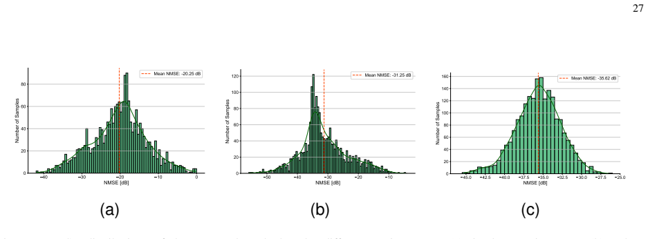
[Tables III and IV; Section VI-E] The same UMi configuration is reported as -50.71 dB mean CFR-NMSE in Table III but -35.76 dB in Table IV. Fig. 6 text reports UMa -21.2 dB, InF -29.8 dB, CDL-A -35.7 dB, while Table III lists -20.25, -31.25, -35.76 dB. The abstract's headline '3.13 to 12.22 dB improvement' and the conclusion's '10.0 to 11.1 dB at UMa' cannot be uniquely derived from these numbers. Please specify for each reported row the exact K, CR, array geometry, and whether the number comes from Fig. 6, Table III, or Table IV, and reconcile the discrepancies.
[Fig. 9 and Section VI-D/VI-G] The cross-domain zero-shot matrix shows off-diagonal entries far better than same-domain entries, e.g., the InF-trained model achieves -77.76 dB on InH vs -23.92 dB on InF, and the UMi-trained model achieves -77.35 dB on InH vs -35.61 dB on UMi. This is internally inconsistent with the expectation that a model evaluated on its own training environment should perform at least as well. Section VI-D explicitly permits environment-appropriate K, so the comparison may use different K per target environment; that is not zero-shot in the strong sense claimed in the abstract. Either fix the evaluation protocol (fixed K or report K per cell) or temper the zero-shot claim. Additionally, Section VI-G introduces 'inference-time time-of-flight alignment' without any algorithmic description; define or remove it.
[Abstract and Section VI-I] The claimed 2700x speedup over OMP and 6400x over LASSO is not supported by Table IV. Using the table's runtimes, 630.15 ms / 0.6239 ms ≈ 1010x for UMa and 630.15 / 0.4824 ≈ 1306x for InF; for LASSO, 88648.56 / 0.6239 ≈ 142,000x, not 6400x. Please recalculate and report the actual ratios, and state the exact TAP configuration used for each speedup.
[Section V-D and Section VI-I] The paper claims 'true architecture independence' and suggests constant computational cost across array sizes. While DelayNet's parameter count is independent of Nant, the LS solver Eq. (24) and the FLOP formula in Section VI-I scale linearly with Nant through the terms 8K Nsc Nant and 8K^2 Nant. Thus the claim of constant computational cost is not accurate. Please qualify the claim as parameter-count independence and report how runtime and FLOPs scale with antenna count.

minor comments (5)

[Section IV-B3] The phrase 'become exponentially more destructive' with bandwidth is inaccurate: Eq. (19) gives polynomial growth (quadratic in Delta tau and O(E_f), with f_k linear). Suggest replacing with 'increasingly destructive' or a precise asymptotic statement.
[Abstract and Algorithm 2] The abstract says the BS reconstructs via a 'simple inverse fast Fourier transform', but Algorithm 2 forms a dictionary A from the estimated delays and multiplies A X. Unless the delays are grid-aligned, this is a non-uniform inverse Fourier transform, not a standard IFFT. Clarify the wording.
[Section II-D] The claim that 'constant parameter counts and computational costs across varying antenna array sizes remains an open challenge' is contradicted by the paper's own LS solver scaling; see the corresponding major comment.
[Fig. 6] The y-axis of Fig. 6 is labeled 'NMSE [dB]' with positive values, while the text quotes negative dB values. Please invert the sign or relabel the axis to avoid confusion.
[Eq. (25)] The heatmap target in Eq. (25) uses ray-tracing amplitudes alpha_l. For the CDL-A stochastic environment, clarify how these amplitudes are obtained and whether the same target generation is meaningful for a stochastic channel model.

Circularity Check

0 steps flagged · score 0.0 of 10

No significant circularity: the TAP pipeline is self-contained and benchmarked against external baselines.

full rationale

The paper's derivation chain is not circular under the definitions used here. TAP's reconstruction is a projection of the current CFR onto the subspace spanned by the estimated delays: \hat{H} = A (A^H A + \lambda I)^{-1} A^H H_tgt. Nothing in this chain is preset by construction to equal the reported CFR-NMSE; the end-to-end loss functions are used only for training, and evaluation is on held-out test sets against external baselines (CsiNet, OMP, LASSO, TVAL3, codebooks). The heatmap supervision L_heatmap uses oracle delays from the ray-tracing simulator, but that is ordinary supervised training, not a by-construction equivalence: the network still must generalize to held-out samples, and the LS amplitudes are computed from the current target channel, not from labels. The only same-author citation, [31] (H. Joo, S. Choi, S. Ryu, H. J. Yang), appears in the related-work survey and is not load-bearing for any theorem, architecture choice, or performance claim. Section VII's far-field limitation is a disclosed modeling assumption with a derived error bound, not a circular step. The internal inconsistencies between Fig. 9 and Tables III/IV are correctness/consistency concerns, not circularity under the required definition, because they do not show that any prediction reduces to its inputs by construction. No specific reduction (Eq. X = Eq. Y by construction, or a fitted parameter renamed as a prediction) can be exhibited in this paper.

Assumptions & free parameters 4 free parameters · 7 assumptions · 1 invented entities

The system rests on two physical premises (delay-domain sparsity and far-field shared delays), one statistical premise (delay smoothness over the temporal window), and one training-data premise (oracle path parameters from the simulator). The far-field premise is the most fragile: Section VII shows the LS solver cannot correct the frequency-dependent phase ramp that near-field wavefronts introduce. The oracle-label premise matters for deployment because real CSI feedback has no access to true path delays except through estimation. No new physical entities are introduced; the only coined mechanism, 'inference-time time-of-flight alignment' (Section VI-G), appears once without definition.

free parameters (4)

K (number of estimated paths) = 20 (UMa), 40 (CDL-A), 90 (InF)
Chosen per environment so that K paths capture 95% of channel energy (Eq. 30). Directly sets CR and NMSE, and makes cross-environment comparisons operate at different compression ratios.
sigma (heatmap Gaussian width) = not reported
Hand-chosen width of the Gaussian target in Eq. (25); controls the sharpness of delay supervision and is never quantified.
lambda (LS regularization) = not reported
Regularization in Eq. (24); affects amplitude estimation and NMSE; value not given.
W (temporal window length) = 9 for UMa/InF/UMi/InH; 1 for CDL-A
Chosen by hand; the paper uses CDL-A with W=1 as an ablation to attribute part of the noise resilience to temporal history.

assumptions (7)

domain assumption Far-field planar wavefront: all antennas share identical multipath delays; spatial differences collapse into per-antenna complex amplitudes
Section III; the dictionary construction and antenna-averaged DelayNet rely on joint-spatial sparsity. Section VII shows that if it fails (near-field), the LS solver cannot compensate the residual phase ramp in Eq. (34).
domain assumption Delay-domain sparsity: the CIR is K-sparse with K much smaller than N_sc
Section III; basis of the compressed feedback rate and of choosing a finite path set.
domain assumption Delay profile temporal smoothness: propagation delays evolve slowly over W consecutive slots
Section III and V-A; the temporal input window is the paper's main denoising and disambiguation mechanism.
domain assumption Oracle training labels: true delays and amplitudes are available from the ray-tracing simulator to build the heatmap target
Section V-F, Eq. (25). In real deployments only noisy observed CFRs exist; the paper does not show whether L_CFR-only training recovers performance.
domain assumption Hamming windowing suppresses sinc sidelobes enough to eliminate phantom peaks
Section V-A; the paper argues windowing replaces OMP's iterative interference cancellation, but no quantitative ablation supports this directly.
domain assumption Simulated 3GPP environments (Sionna RT, DeepMIMO, CDL) are representative for the zero-shot generalization claims
All evaluations and generalization claims rest on five simulation datasets (Section VI-A); no over-the-air validation.
standard math Standard OFDM and pilot model with orthogonal pilots and AWGN
Eqs. (1)-(5); used to relate CSI-RS SNR to input noise.

invented entities (1)

Inference-time time-of-flight alignment
purpose: Invoked as the mechanism that enables zero-shot cross-environment transfer in Section VI-G
Mentioned once in Section VI-G as the enabler of zero-shot transfer; never defined, derived, or ablated anywhere in the paper. As printed it is an unexplained mechanism attached to a headline claim.

how reviews work

0 comments

Cite this review

Pith. "Pith review of Temporal Channel Estimation for Generalized CSI Feedback." pith.science (2026). https://pith.science/paper/N3MEUAJO

@misc{pith2026260801713,
  author       = {Pith},
  title        = {Pith review of: Temporal Channel Estimation for Generalized CSI Feedback},
  year         = {2026},
  howpublished = {\url{https://pith.science/paper/N3MEUAJO}},
  note         = {Machine review of arXiv:2608.01713}
}

read the original abstract

Efficient Channel State Information (CSI) feedback is indispensable for frequency division duplex (FDD) massive multiple-input multiple-output (MIMO) systems. Existing compressed sensing (CS) algorithms exploit delay-domain sparsity but suffer from prohibitive iterative latency and discrete grid mismatch. Conversely, deep learning (DL) approaches achieve rapid inference but lack spatial scalability and domain adaptability, failing to generalize to unseen propagation environments, and demand computationally heavy encoders and decoder. In this paper, we propose TAP, a Tap-Assisted Parametric CSI Compression. TAP is a one-shot neural framework that unifies the speed of DL with the mathematical interpretability of CS. TAP replaces iterative pursuit with a lightweight 1D neural network that extracts dominant continuous propagation delays from temporal channel sequences via a differentiable sub-grid interpolation operator. TAP achieves true architecture independence, enabling zero-shot generalization across diverse array geometries and unseen propagation environments. Furthermore, TAP yields a completely decoder-free payload, allowing the BS to reconstruct the channel via a simple inverse fast Fourier transform (IFFT). Extensive evaluations across five 3GPP environments demonstrate that TAP achieves a 3.13 to 12.22 dB channel frequency response normalized mean square error (CFR-NMSE) improvement over CsiNet while shrinking the model footprint by 660 times to under 1 MB. Operating with sub-millisecond latencies, TAP accelerates inference by 2700 times over classical iterative OMP, providing a scalable and deployment-ready solution for next-generation networks.

Figures

Figures reproduced from arXiv: 2608.01713 by the authors.

**Figure 2.** NMSE and latency of OMP-based CSI compression under different number of estimated taps. [PITH_FULL_IMAGE:figures/full_fig_p012_2.png] view at source ↗

**Figure 3.** Pipeline of TAP. • Amplitude Weighting: The reconstruction error is weighted by the true tap amplitudes |ai |. A minuscule delay error ∆τ on a dominant line-of-sight (LoS) path will severely degrade the overall CFR-NMSE, regardless of the precision of the complex coefficient optimization. These fundamental limitations, namely prohibitive iterative complexity, vulnerability to spectral leakage, discrete dictionary m… view at source ↗

Figures from the paper (10 more)

**Figure 4.** Figure 4: CIR plots of different environments: (a) Outdoor environment; (b) Indoor environment. [PITH_FULL_IMAGE:figures/full_fig_p025_4.png]

**Figure 5.** Figure 5: Cumulative distribution function (CDF) of the required number of delay bins to capture 95% of the total channel energy [PITH_FULL_IMAGE:figures/full_fig_p026_5.png]

**Figure 6.** Figure 6: NMSE distributions of the proposed method under different environments. [PITH_FULL_IMAGE:figures/full_fig_p026_6.png]

**Figure 7.** Figure 7: NMSE distributions of the proposed method under different environments; (a) Outdoor environment; (b) Indoor [PITH_FULL_IMAGE:figures/full_fig_p027_7.png]

**Figure 8.** Figure 8: Pareto efficiency graph of the proposed method under different environments; (a) UMa environment; (b) InF environment. [PITH_FULL_IMAGE:figures/full_fig_p028_8.png]

**Figure 9.** Figure 9: Cross-domain zero-shot generalization performance matrix between different environments. [PITH_FULL_IMAGE:figures/full_fig_p028_9.png]

**Figure 10.** Figure 10: Geometric scalability evaluation: NMSE performance across heterogeneous antenna array geometries; (a) Outdoor [PITH_FULL_IMAGE:figures/full_fig_p029_10.png]

**Figure 11.** Figure 11: Downlink achievable spectral efficiency (bps/Hz) in the CDL-A environment using a linear precoder derived from the [PITH_FULL_IMAGE:figures/full_fig_p031_11.png]

**Figure 12.** Figure 12: Impact of payload quantization on reconstruction NMSE across different bit-widths for the CDL-A dataset. TAP [PITH_FULL_IMAGE:figures/full_fig_p032_12.png]

**Figure 13.** Figure 13: Impact of CSI-RS estimation noise at the receiver. The reconstruction NMSE is evaluated against varying input CSI-RS [PITH_FULL_IMAGE:figures/full_fig_p033_13.png]

Discussion (0). Continue with ORCID to comment.

Reference graph

Works this paper leans on

44 extracted references · 38 canonical work pages

[1]

Joint channel training and feedback for FDD massive MIMO systems,

W. Shen, L. Dai, Y . Shi, B. Shim, and Z. Wang, “Joint channel training and feedback for FDD massive MIMO systems,” IEEE Trans. Veh. Technol., vol. 65, no. 10, pp. 8762–8767, 2016

work page 2016
[2]

Orthogonal matching pursuit: recursive function approximation with applications to wavelet decomposition,

Y . Pati, R. Rezaiifar, and P. Krishnaprasad, “Orthogonal matching pursuit: recursive function approximation with applications to wavelet decomposition,” inProc. Asilomar Conf. Signal Syst. Comput., 1993, pp. 40–44 vol.1

work page 1993
[3]

Signal recovery from random measurements via orthogonal matching pursuit,

J. A. Tropp and A. C. Gilbert, “Signal recovery from random measurements via orthogonal matching pursuit,”IEEE Trans. Inform. Theory, vol. 53, no. 12, pp. 4655–4666, 2007

work page 2007
[4]

Sparse channel estimation based on compressed sensing for massive MIMO systems,

C. Qi, Y . Huang, S. Jin, and L. Wu, “Sparse channel estimation based on compressed sensing for massive MIMO systems,” inProc. IEEE Int. Conf. Commun. (ICC), 2015, pp. 4558–4563

work page 2015
[5]

Beam-blocked channel estimation for FDD massive MIMO with compressed feedback,

W. Huang, Y . Huang, W. Xu, and L. Yang, “Beam-blocked channel estimation for FDD massive MIMO with compressed feedback,”IEEE Access, vol. 5, pp. 11 791–11 804, 2017

work page 2017
[6]

Deep learning and compressive sensing-based CSI feedback in FDD massive MIMO systems,

P. Liang, J. Fan, W. Shen, Z. Qin, and G. Y . Li, “Deep learning and compressive sensing-based CSI feedback in FDD massive MIMO systems,”IEEE Trans. Veh. Technol., vol. 69, no. 8, pp. 9217–9222, 2020

work page 2020
[7]

An efficient augmented lagrangian method with applications to total variation minimization,

C. Li, W. Yin, H. Jiang, and Y . Zhang, “An efficient augmented lagrangian method with applications to total variation minimization,”Comput. Optim. Appl., vol. 56, no. 3, pp. 507–530, December 2013

work page 2013
[8]

Deep convolutional compression for massive MIMO CSI feedback,

Q. Yang, M. B. Mashhadi, and D. G ¨und¨uz, “Deep convolutional compression for massive MIMO CSI feedback,” inProc. IEEE Int. Workshop Mach. Learn. Signal Process (MLSP), 2019, pp. 1–6. 36

work page 2019

Show all 44 references

[9]

Deep learning for massive MIMO CSI feedback,

C.-K. Wen, W.-T. Shih, and S. Jin, “Deep learning for massive MIMO CSI feedback,”IEEE Wireless Commun. Lett., vol. 7, no. 5, pp. 748–751, 2018

2018
[10]

NR; Physical layer procedures for data,

3GPP, “NR; Physical layer procedures for data,” 3rd Generation Partnership Project (3GPP), Technical Specification (TS) 38.214, Jun. 2026, V19.4.0

2026
[11]

Multi-resolution CSI feedback with deep learning in massive MIMO system,

Z. Lu, J. Wang, and J. Song, “Multi-resolution CSI feedback with deep learning in massive MIMO system,” inProc. IEEE Int. Conf. Commun. (ICC), 2020, pp. 1–6

2020
[12]

Deep learning-based CSI feedback approach for time-varying massive MIMO channels,

T. Wang, C.-K. Wen, S. Jin, and G. Y . Li, “Deep learning-based CSI feedback approach for time-varying massive MIMO channels,”IEEE Wireless Commun. Lett., vol. 8, no. 2, pp. 416–419, 2019

2019
[13]

Transformer empowered csi feedback for massive MIMO systems,

Y . Xu, M. Yuan, and M.-O. Pun, “Transformer empowered csi feedback for massive MIMO systems,” inProc. Wireless Opt. Commun. Conf. (WOCC), 2021, pp. 157–161

2021
[14]

Transnet: Full attention network for CSI feedback in FDD massive MIMO system,

Y . Cui, A. Guo, and C. Song, “Transnet: Full attention network for CSI feedback in FDD massive MIMO system,”IEEE Wireless Commun. Lett., vol. 11, no. 5, pp. 903–907, 2022

2022
[15]

DD-transnet-based CSI feedback in imperfect channel estimation in MIMO-OTFS systems for V2I scenarios,

Y . Liao and Y . Luo, “DD-transnet-based CSI feedback in imperfect channel estimation in MIMO-OTFS systems for V2I scenarios,”IEEE Trans. Intell. Transport. Syst., vol. 26, no. 11, pp. 18 839–18 853, 2025

2025
[16]

Transformer-assisted parametric CSI feedback for mmwave massive MIMO systems,

H. Ju, S. Jeong, S. Kim, B. Lee, and B. Shim, “Transformer-assisted parametric CSI feedback for mmwave massive MIMO systems,”IEEE Trans. Wireless Commun., vol. 23, no. 12, pp. 18 774–18 787, 2024

2024
[17]

Mixed-timescale deep-unfolding for joint channel estimation and hybrid beamforming,

K. Kang, Q. Hu, Y . Cai, G. Yu, J. Hoydis, and Y . C. Eldar, “Mixed-timescale deep-unfolding for joint channel estimation and hybrid beamforming,”IEEE J. Sel. Areas Commun., vol. 40, no. 9, pp. 2510–2528, 2022

2022
[18]

Data-driven estimation of sinusoid frequencies,

G. Izacard, S. Mohan, and C. Fernandez-Granda, “Data-driven estimation of sinusoid frequencies,” inProc. Advances Neural Inf. Process. Syst. (NeurIPS), 2019

2019
[19]

Compressed sensing for wireless communications: Useful tips and tricks,

J. W. Choi, B. Shim, Y . Ding, B. Rao, and D. I. Kim, “Compressed sensing for wireless communications: Useful tips and tricks,”IEEE Commun. Surveys Tuts., vol. 19, no. 3, pp. 1527–1550, 2017

2017
[20]

Compressive sensing based channel feedback protocols for spatially-correlated massive antenna arrays,

P.-H. Kuo, H. T. Kung, and P.-A. Ting, “Compressive sensing based channel feedback protocols for spatially-correlated massive antenna arrays,” inProc. IEEE Wireless Commun. Netw. Conf. (WCNC), 2012, pp. 492–497

2012
[21]

Model-based compressive sensing,

R. G. Baraniuk, V . Cevher, M. F. Duarte, and C. Hegde, “Model-based compressive sensing,”IEEE Trans. Inform. Theory, vol. 56, no. 4, pp. 1982–2001, 2010

1982
[22]

Bayesian compressive sensing,

S. Ji, Y . Xue, and L. Carin, “Bayesian compressive sensing,”IEEE Trans. Signal Processing, vol. 56, no. 6, pp. 2346–2356, 2008

2008
[23]

Spatially common sparsity based adaptive channel estimation and feedback for FDD massive MIMO,

Z. Gao, L. Dai, Z. Wang, and S. Chen, “Spatially common sparsity based adaptive channel estimation and feedback for FDD massive MIMO,”IEEE Trans. Signal Processing, vol. 63, no. 23, pp. 6169–6183, 2015

2015
[24]

Angle-delay domain hybrid model-driven and data-driven downlink CSI acquisition for FDD massive MIMO systems,

X. He, H. Hou, T. Fang, W. Wang, and S. Jin, “Angle-delay domain hybrid model-driven and data-driven downlink CSI acquisition for FDD massive MIMO systems,”IEEE Trans. Veh. Technol., vol. 74, no. 1, pp. 1788–1793, 2025

2025
[25]

Downlink CSI feedback algorithm with deep transfer learning for FDD massive MIMO systems,

J. Zeng, J. Sun, G. Gui, B. Adebisi, T. Ohtsuki, H. Gacanin, and H. Sari, “Downlink CSI feedback algorithm with deep transfer learning for FDD massive MIMO systems,”IEEE Trans. Cogn. Commun. Netw., vol. 7, no. 4, pp. 1253–1265, 2021

2021
[26]

DDA-Net: A discrepancy-based domain adaptation network for CSI feedback transferability,

Y . Feng, C. Ye, R. Li, H. Pan, and D. Korpi, “DDA-Net: A discrepancy-based domain adaptation network for CSI feedback transferability,” inProc. IEEE Int. Conf. Commun. (ICC), 2023, pp. 4157–4162

2023
[27]

Dynamically fine-tuned neural compressor for FDD massive MIMO CSI feedback,

M. Sattari, D. G ¨und¨uz, and T. Svensson, “Dynamically fine-tuned neural compressor for FDD massive MIMO CSI feedback,” inProc. IEEE. Int. Workshop Signal Process. Artif. Intell. Wireless Commun. (SPAWC), 2025, pp. 1–5. 37

2025
[28]

A knowledge-driven meta-learning method for CSI feedback,

H. Xiao, W. Tian, W. Liu, Z. Zhang, Z. Shi, L. Guo, and J. Shen, “A knowledge-driven meta-learning method for CSI feedback,” inProc. IEEE Int. Conf. Commun. (ICC), 2023, pp. 4138–4143

2023
[29]

Deep learning for efficient CSI feedback in massive MIMO: Adapting to new environments and small datasets,

Z. Liu, L. Wang, L. Xu, and Z. Ding, “Deep learning for efficient CSI feedback in massive MIMO: Adapting to new environments and small datasets,”IEEE Trans. Wireless Commun., vol. 23, no. 9, pp. 12 297–12 312, 2024

2024
[30]

Unsupervised adversarial domain adaptation for CSI feedback in codeword feature space,

J. Chen, X. Gu, H. Li, and Z. Liu, “Unsupervised adversarial domain adaptation for CSI feedback in codeword feature space,” inProc. Int. Conf. Commun. Inf. Process., 2026, p. 269–273

2026
[31]

Compressed-CSI feedback with near real-time domain adaptation,

H. Joo, S. Choi, S. Ryu, and H. J. Yang, “Compressed-CSI feedback with near real-time domain adaptation,”IEEE Trans. Commun., pp. 1–1, 2026

2026
[32]

Generalizable learning for massive MIMO CSI feedback in unseen environments,

H. Wang, Z. Sun, S. Han, X. Wang, and Z. Wang, “Generalizable learning for massive MIMO CSI feedback in unseen environments,”IEEE Trans. Wireless Commun., vol. 25, pp. 12 514–12 530, 2026

2026
[33]

Deep learning based antenna selection for MIMO SDR system,

S. Zhong, H. Feng, P. Zhang, J. Xu, H. Luo, J. Zhang, T. Yuan, and L. Huang, “Deep learning based antenna selection for MIMO SDR system,”Sensors, vol. 20, no. 23, 2020

2020
[34]

Learning-based joint channel prediction and antenna selection for massive MIMO with partial CSI,

K. He, T. X. Vu, S. Chatzinotas, and B. Ottersten, “Learning-based joint channel prediction and antenna selection for massive MIMO with partial CSI,” inProc. IEEE Globecom Workshops (GC Wkshps), 2022, pp. 178–183

2022
[35]

Towards CSI-native foundation models: A channel-adaptive roadmap for 6G,

C. Zhang, X. Lyu, C. Ren, S. Liu, and Q. Cui, “Towards CSI-native foundation models: A channel-adaptive roadmap for 6G,” 2026,arXiv:2606.20670

2026 arXiv
[36]

A low-complexity orthogonal matching pursuit algorithm based on multi-scale multi-lag underwater acoustic channels,

J. Du, Y . Yan, and X. Li, “A low-complexity orthogonal matching pursuit algorithm based on multi-scale multi-lag underwater acoustic channels,” inProc. IEEE Int. Conf. Signal Process. Commun. Comput (ICSPCC), 2024, pp. 1–6

2024
[37]

Remodelled and reduced complexity-OMP-based channel estimation schemes for intelligent reflecting surface-aided millimeter wave systems,

O. O. Oyerinde, A. Flizikowski, and T. Marciniak, “Remodelled and reduced complexity-OMP-based channel estimation schemes for intelligent reflecting surface-aided millimeter wave systems,” inProc. Int. Conf. Signal Process. Commun. Syst. (ICSPCS), 2023, pp. 1–5

2023
[38]

Average performance of OMP and thresholding under dictionary mismatch,

M.-C. Pali, S. Ruetz, and K. Schnass, “Average performance of OMP and thresholding under dictionary mismatch,”IEEE Signal Processing Lett., vol. 29, pp. 1077–1081, 2022

2022
[39]

Gridless parameter estimation for one-bit MIMO radar with time-varying thresholds,

F. Xi, Y . Xiang, S. Chen, and A. Nehorai, “Gridless parameter estimation for one-bit MIMO radar with time-varying thresholds,”IEEE Trans. Signal Processing, vol. 68, pp. 1048–1063, 2020

2020
[40]

NR; User Equipment (UE) radio transmission and reception; Part 1: Range 1 Standalone,

3GPP, “NR; User Equipment (UE) radio transmission and reception; Part 1: Range 1 Standalone,” 3rd Generation Partnership Project (3GPP), Technical Specification (TS) 38.101-1, Jul. 2026, V20.0.0

2026
[41]

Study on channel model for frequencies from 0.5 to 100 GHz,

——, “Study on channel model for frequencies from 0.5 to 100 GHz,” 3rd Generation Partnership Project (3GPP), Technical Report (TR) 38.901, Jun. 2026, V19.4.0

2026
[42]

Sionna RT: Differentiable ray tracing for radio propagation modeling,

J. Hoydis, F. A. Aoudia, S. Cammerer, M. Nimier-David, N. Binder, G. Marcus, and A. Keller, “Sionna RT: Differentiable ray tracing for radio propagation modeling,” 2023,arXiv:2303.11103

2023 arXiv
[43]

Sionna: An open-source library for next-generation physical layer research,

J. Hoydis, S. Cammerer, F. A. Aoudia, A. Vem, N. Binder, G. Marcus, and A. Keller, “Sionna: An open-source library for next-generation physical layer research,” 2023,arXiv:2203.11854

2023 arXiv
[44]

DeepMIMO: A generic deep learning dataset for millimeter wave and massive MIMO applications,

A. Alkhateeb, “DeepMIMO: A generic deep learning dataset for millimeter wave and massive MIMO applications,” 2019, arXiv:1902.06435

2019 arXiv

Pith tools

Reviewed August 4, 2026 · model on record in the stance chip above.

[1] [1]

Joint channel training and feedback for FDD massive MIMO systems,

W. Shen, L. Dai, Y . Shi, B. Shim, and Z. Wang, “Joint channel training and feedback for FDD massive MIMO systems,” IEEE Trans. Veh. Technol., vol. 65, no. 10, pp. 8762–8767, 2016

work page 2016

[2] [2]

Orthogonal matching pursuit: recursive function approximation with applications to wavelet decomposition,

Y . Pati, R. Rezaiifar, and P. Krishnaprasad, “Orthogonal matching pursuit: recursive function approximation with applications to wavelet decomposition,” inProc. Asilomar Conf. Signal Syst. Comput., 1993, pp. 40–44 vol.1

work page 1993

[3] [3]

Signal recovery from random measurements via orthogonal matching pursuit,

J. A. Tropp and A. C. Gilbert, “Signal recovery from random measurements via orthogonal matching pursuit,”IEEE Trans. Inform. Theory, vol. 53, no. 12, pp. 4655–4666, 2007

work page 2007

[4] [4]

Sparse channel estimation based on compressed sensing for massive MIMO systems,

C. Qi, Y . Huang, S. Jin, and L. Wu, “Sparse channel estimation based on compressed sensing for massive MIMO systems,” inProc. IEEE Int. Conf. Commun. (ICC), 2015, pp. 4558–4563

work page 2015

[5] [5]

Beam-blocked channel estimation for FDD massive MIMO with compressed feedback,

W. Huang, Y . Huang, W. Xu, and L. Yang, “Beam-blocked channel estimation for FDD massive MIMO with compressed feedback,”IEEE Access, vol. 5, pp. 11 791–11 804, 2017

work page 2017

[6] [6]

Deep learning and compressive sensing-based CSI feedback in FDD massive MIMO systems,

P. Liang, J. Fan, W. Shen, Z. Qin, and G. Y . Li, “Deep learning and compressive sensing-based CSI feedback in FDD massive MIMO systems,”IEEE Trans. Veh. Technol., vol. 69, no. 8, pp. 9217–9222, 2020

work page 2020

[7] [7]

An efficient augmented lagrangian method with applications to total variation minimization,

C. Li, W. Yin, H. Jiang, and Y . Zhang, “An efficient augmented lagrangian method with applications to total variation minimization,”Comput. Optim. Appl., vol. 56, no. 3, pp. 507–530, December 2013

work page 2013

[8] [8]

Deep convolutional compression for massive MIMO CSI feedback,

Q. Yang, M. B. Mashhadi, and D. G ¨und¨uz, “Deep convolutional compression for massive MIMO CSI feedback,” inProc. IEEE Int. Workshop Mach. Learn. Signal Process (MLSP), 2019, pp. 1–6. 36

work page 2019