REVIEW 2 major objections 5 minor 68 references
Dynamically suppressing cavity dephasing induced by frequency fluctuations of a coupled nonlinear mode
T0 review · 2 major / 5 minor · reviewed 2026-08-15 · deepseek-v4-flash
Pith's one-line read A weak detuned drive on a transmon cancels the flux-noise dephasing it imposes on a coupled cavity, lifting the cavity dephasing time from about 0.1 ms to about 2 ms.
desk verdict SAFE is a clever and well-analyzed drive-only protocol for protecting cavities from flux noise, but the headline 20x dephasing improvement rests on a 5-μs exponential fit that does not rule out a longer-time residual. read the letter →
The pith
A machine-rendered reading of the paper's core claim, the machinery that carries it, and where it could break.
The reading
What carries the argument
The load-bearing object is the rotating-frame Hamiltonian $H_R = \Delta_{\rm bd} b^\dagger b + (K/2) b^{\dagger 2} b^2 + \omega_c c^\dagger c + \chi b^\dagger b c^\dagger c + \Omega_0(b+b^\dagger)$ together with its perturbative eigenvalues, which give the shifted cavity transition frequency $\tilde{\omega}_{c;n,m}$ and its flux susceptibility $D_{n,m} = \partial \tilde{\omega}_{c;n,m}/\partial\Phi$. The cancellation works because both the static Lamb shift (proportional to $g^2/\Delta_{bc}^2$) and the drive-induced Stark shift (proportional to $\Omega_0^2 \chi/\Delta_{\rm bd}^2$) fluctuate with the transmon frequency $\partial\omega_b/\partial\Phi$; choosing $\Delta_{\rm bd}=(4\Omega_0^2 K)^{1/3}$ makes the two contributions cancel to first order. The paper supplements this with an effective Lindblad master equation, derived by Schrieffer–Wolff transformation and two-level truncation, whose residual pure-dephasing rate $\Gamma_{c\phi}^{\rm ss} = (\partial\omega_b/\partial\Phi)^2 A^2/(4|K/2\pi|) + (\gamma_{b\downarrow}/16)(\Delta_{\rm bd}/K)^2 + \gamma_{b\uparrow}$ quantifies the floor at the sweet spot and sets the trade-off between the number of protected Fock levels and the suppression factor.
What would settle it
Measure the cavity coherence time with the SAFE drive at $\Delta_{\rm bd}=(4\Omega_0^2 K)^{1/3}$ on a 3D cavity–FTT device with $1/f$ flux-noise amplitude near $10^{-5}\Phi_0$, and extend the Ramsey measurement well beyond the 5 $\mu$s fitting window, to hundreds of microseconds or longer. If the decay remains exponential with $T_2\approx 2$ ms, the extrapolation holds; if a Gaussian or quadratic low-frequency component appears and the apparent $T_\phi$ shortens, the claimed suppression factor is not sustained.
Extended reading notes
Core claim
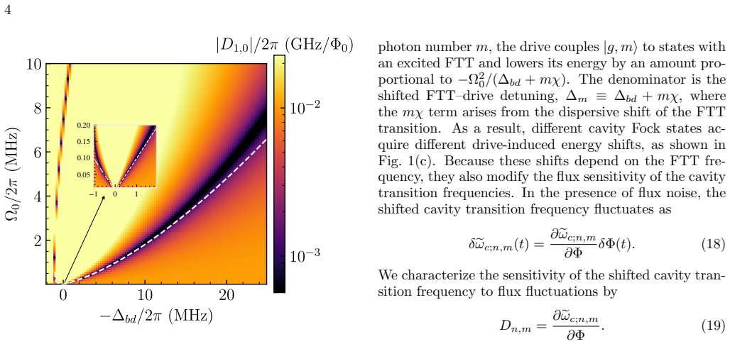
SAFE's central discovery is that a continuous off-resonant drive applied to the nonlinear element can undo the dephasing that the same element's flux noise imposes on a dispersively coupled cavity. Because the dispersive shift makes the drive detuning photon-number dependent ($\Delta_{\rm bd}+m\chi$ for cavity state $|m\rangle$), different Fock states acquire different AC Stark shifts, and the shifted cavity transition frequency $\tilde{\omega}_{c;n,m} = (n-m)(\omega_c - g^2/\Delta_{bc}) - \Omega_0^2/(\Delta_{\rm bd}+n\chi) + \Omega_0^2/(\Delta_{\rm bd}+m\chi)$ acquires a flux dependence that can cancel the Lamb-shift contribution $(g^2/\Delta_{bc}^2)\,\delta\omega_b(t)$. Tuning the drive detuning to $\Delta_{\rm bd} = (4\Omega_0^2 K)^{1/3}$ (large-detuning regime) renders the transition frequency first-order insensitive to flux fluctuations, $D_{n,m}=0$, simultaneously for many Fock-state pairs; a separate condition $\Delta_{\rm bd} = \pm|\Delta_{bc}/g|\,\Omega_0$ protects a specific transition in the small-detuning regime. With representative 3D-cavity/FTT parameters and $1/f$ flux noise of amplitude $10^{-5}\Phi_0$, the paper's simulations show the cavity pure-dephasing time increasing from roughly 0.1 ms to 2 ms, and show that the same sweet spot suppresses logical dephasing in binomial and dual-rail encodings by about an order of magnitude without changing the erasure or photon-loss rate.
Load-bearing premise
The reported 20-fold suppression assumes that the residual dephasing seen in a 5-microsecond simulation window is the full story, meaning the coherence there is set by the Markovian channels of the effective master equation and continues to decay exponentially to the extracted 2 ms, with no slower unmodeled low-frequency or non-Markovian noise tail taking over at longer times.
Editorial extensions
If this is right
- A single drive setting $\Delta_{\rm bd}=(4\Omega_0^2 K)^{1/3}$ simultaneously protects many Fock-state transition frequencies, so encodings like binomial codes that use several Fock-state coherences are protected without re-tuning per transition.
- The cavity relaxation time and the photon-loss/erasure rate are essentially unchanged by the drive, so the photon-loss bias that cat, dual-rail, and binomial codes rely on is preserved while the dephasing channel is suppressed.
- The residual pure-dephasing floor $\Gamma_{c\phi}^{\rm ss}$ grows with $\gamma_{b\downarrow}(\Delta_{\rm bd}/K)^2$, so reducing transmon relaxation or increasing anharmonicity $|K|$ directly improves the cavity dephasing time at the sweet spot.
- A single driven transmon can act as a shared noise shield for multiple cavity modes, as demonstrated for a two-dual-rail-qubit Bell state, where logical dephasing is suppressed by about an order of magnitude and the decoherence-induced infidelity drops from 0.18 to 0.011.
- Drive-induced side effects are subdominant in the analysis: drive-amplitude noise alone would limit $T_\phi$ to about 25 ms for one representative AWG platform, well above the 2 ms demonstrated.
Reading between the lines
- The cancellation mechanism is not obviously restricted to transmon–cavity systems; a plausible extension is that any flux-tunable nonlinear coupler with a photon-number-dependent dispersive shift can be Stark-protected, making SAFE a general tool for shielding bosonic modes behind noise-prone couplers.
- Because the sweet spot is created dynamically, a device could idle at a flux-bias point that is otherwise useful for parametric interactions rather than returning to a static sweet spot, a freedom the paper only gestures toward.
- If the extrapolated 2 ms survives experimental scrutiny, SAFE could be combined with other protection techniques, such as two-tone drives or dynamical decoupling, to push residual dephasing toward the drive-amplitude-noise floor of tens of milliseconds.
- A sharp test of the theory is the predicted non-monotonic dependence of the suppression factor on noise amplitude, with a maximum of roughly $\eta\approx 22$ near $A\approx 6\times 10^{-6}\Phi_0$; measuring $\eta(A)$ on a single device would discriminate the model from a generic dephasing-suppression story.
Signed reviews
Editorial analysis
A structured set of objections, weighed in public.
Referee Report
Summary. The paper introduces SAFE (Stark-Assisted Flux-noise Evasion), a protocol that applies a weak off-resonant microwave drive to a flux-tunable transmon dispersively coupled to a cavity, creating a dynamical sweet spot at which the dressed cavity transition frequency is first-order insensitive to 1/f flux noise. In the large-detuning regime the authors derive the simple condition Δbd = (4Ω0^2 K)^{1/3}, compute the residual Markovian dephasing channels, and support the analytical results with exact Floquet calculations and Monte Carlo simulations of the full Hamiltonian. They report an approximately 20-fold improvement in cavity pure-dephasing time (from about 0.1 ms to about 2 ms) and show that the same drive simultaneously protects multiple Fock-state coherences and multiple cavity modes, with applications to binomial and dual-rail encodings.
Significance. If the quantitative claims hold, SAFE is a practically attractive and hardware-efficient way to preserve the photon-loss bias of bosonic error-correcting codes while operating the nonlinear element away from its static flux sweet spot. The central sweet-spot condition is derived rather than fit, and the paper's key qualitative predictions are checked against independent Floquet numerics and Monte Carlo trajectory simulations. The extension to simultaneous protection of several Fock-state pairs and several cavity modes is a useful advance over single-transition dynamical sweet-spot schemes. The main quantitative claim, however, rests on an extrapolation from a very short coherence window, and the manuscript would be substantially strengthened by a longer-time numerical check or an analytical bound on the second-order flux-noise channel.
major comments (2)
- [Sec. III C, Fig. 3(d), App. G] The headline value Tφ≈2 ms is supported numerically only by a single-exponential fit to the first 5 µs of the ensemble-averaged coherence. At the claimed residual rate Γ≈500–600 s−1, the decay over 5 µs is only about 0.3% of the initial coherence, and the robustness check in App. G extends the window only to 10 µs, still roughly 200 times shorter than the extracted Tφ. The argument that a residual second-order sensitivity would produce a zero-slope quadratic onset only shows that such a component is small over 5–10 µs; it does not establish that its contribution at t≈1 ms is negligible relative to the Markovian channels in Eq. (38). Please extend the trajectory-averaged simulation to a time at which the decay is a measurable few percent, or provide an analytical estimate of the second-order longitudinal dephasing rate (for example, using ∂²ω̃c/∂Φ² and A² ln(ω_uv/ω_ir)) demonstrating that it is subdominant at millisecond times. As written, the 20-fold suppression factor is an extrapolation.
- [Sec. III B, Eq. (38)] Equation (38) is presented as the complete residual pure-dephasing rate at the dynamical sweet spot, but it contains no term representing dephasing from the low-frequency tail of the 1/f spectrum acting through the second- and higher-order flux sensitivity of the dressed cavity frequency. Because SAFE cancels only the first-order susceptibility D_{n,m}=∂ω̃c/∂Φ, the quadratic channel cannot be assumed negligible without a quantitative estimate. The paper should state the time range over which Eq. (38) is expected to hold and provide a bound on the second-order contribution, which is needed to justify the extrapolation from the short-time numerical window to Tφ≈2 ms.
minor comments (5)
- [Sec. III B] The cross-reference "Sec. II B 0 a" appears to be a typo; it should refer to Sec. II B, item a.
- [Sec. III C and App. G] The drive amplitude Ω0 used for the Monte Carlo and time-domain results in Fig. 3 is not stated; only Δbd/2π=−19 MHz is quoted. Please report Ω0 and, if it differs from the value implied by Eq. (22), the exact detuning used in the time-domain simulation, so that the results can be reproduced and compared with Eq. (38).
- [Appendix H, Eq. (H4)] The displayed inequality "τ≫ Ω0/|Δbd|² (22) = sqrt(1/(4KΔbd))" is confusingly formatted because the reference number "(22)" is embedded in the formula. Please rewrite it with the reference placed elsewhere.
- [Abstract and Sec. I] The phrase "1/fflux noise" is missing a space; it should read "1/f flux noise".
- [Appendix E] The stated rescaled coupling g/2π=0.10 GHz is slightly inconsistent with g=g′/(2φ_ZPF) using φ_ZPF≈0.24 and g′/2π=0.050 GHz, which gives about 0.104 GHz. Please clarify the rounding or the exact value of φ_ZPF used.
Circularity Check
No significant circularity: the SAFE sweet-spot condition and residual dephasing rate are derived analytically and then verified by full-Hamiltonian Monte Carlo simulation.
full rationale
The central derivation chain is self-contained rather than self-referential. The shifted cavity transition frequency is obtained from the rotating-frame Hamiltonian H_R (Eq. 16) by perturbation theory, giving Eq. (17); differentiating with respect to flux yields the susceptibility D_n,m (Eqs. 19–21). Setting D_n,m = 0 in the large-detuning regime algebraically produces the sweet-spot detuning Δ_bd = (4Θ_0^2 K)^{1/3} (Eq. 22), and the same procedure yields the small-detuning condition (Eq. 28). The residual cavity pure-dephasing rate at the sweet spot, Eq. (38), is obtained by substituting Eq. (22) into the independently derived rate expression Eq. (37), not by fitting. The numerical confirmation is also independent: Fig. 2 computes the susceptibility from Floquet quasienergies obtained with QuTiP using the full Hamiltonian, and the time-domain dephasing simulation in Sec. III C and App. G evolves the full Hamiltonian H_full with stochastically generated 1/f flux trajectories. The extracted T_φ ≈ 2 ms is an output of those trajectories, not an input to any part of the derivation. The only imported empirical constant is √|ℓn(ω_ir t)| ≈ 4, taken from external experimental work (Ref. [52]), and the flux-noise amplitude A is an external device parameter; neither is a renaming of this paper's own outputs. The authors cite their earlier dynamical-sweet-spot work (Ref. [43], with overlapping authors) for the general principle of continuous-drive sweet spots, but the new cavity-specific protection is derived here and checked against independent simulation, so that self-citation is not load-bearing. App. G's short-window exponential fit (5 μs, doubled to 10 μs) is a possible extrapolation risk for the claimed 2 ms number, but that is a robustness or correctness concern, not circularity: no fitted parameter is renamed as a prediction. Therefore no circular step can be exhibited from the paper's own equations, and the appropriate finding is no significant circularity.
Assumptions & free parameters
assumptions (6)
- domain assumption Transmon regime and dispersive approximation: EC<<EJ, g/|Δbc|<<1, g/|Δbc+K|<<1.
- domain assumption Weak off-resonant drive: Ω0≪|Δbd| and |Δbd|≪|K| in the large-detuning SAFE regime.
- domain assumption 1/f flux noise model with S(ω)=A^2/|ω/2π| and an infrared cutoff.
- domain assumption FTT initialized in its ground state, with k_B T≪ℏω_b so that thermal excitation is negligible.
- domain assumption Markovian approximation for photon-shot noise and drive-induced excitation in Eq. (37).
- domain assumption The two dual-rail cavities are mutually far detuned so FTT-mediated interactions and cross-Kerr terms are negligible.
Cite this review
Pith. "Pith review of Dynamically suppressing cavity dephasing induced by frequency fluctuations of a coupled nonlinear mode." pith.science (2026). https://pith.science/paper/K234443X
@misc{pith2026260804494,
  author       = {Pith},
  title        = {Pith review of: Dynamically suppressing cavity dephasing induced by frequency fluctuations of a coupled nonlinear mode},
  year         = {2026},
  howpublished = {\url{https://pith.science/paper/K234443X}},
  note         = {Machine review of arXiv:2608.04494}
}
abstract
High-coherence superconducting cavities offer a promising platform for quantum information, with long coherence times and negligible intrinsic dephasing. However, cavity control generally relies on nonlinear Josephson elements whose frequency fluctuations are inherited by the cavity as dephasing, potentially limiting control fidelities and eroding the noise bias used in error-correction protocols. Here, we introduce Stark-Assisted Flux-noise Evasion (SAFE), a hardware-efficient protocol that protects the cavity from inherited dephasing using only a weak off-resonant microwave drive applied to the nonlinear element. As a concrete setup, we analyze a 3D superconducting cavity dispersively coupled to a flux-tunable transmon (FTT) subject to $1/f$ flux noise. Analytical predictions are confirmed by Monte Carlo simulations with realistic parameters, which show that SAFE can extend the cavity dephasing time by more than an order of magnitude while keeping residual drive-induced decoherence subdominant.
Figures


Figures from the paper (5 more)


Reference graph
Works this paper leans on
-
[1]
Floquet Theorem Consider a Hilbert spaceHof dimensionNand a time- dependent HamiltonianH(t) with periodτ, satisfying H(t+τ) =H(t). Floquet’s theorem states that the so- lutions to the Schr¨ odinger equation can be written as |ϕn(t)⟩=e −iεnt|ψn(t)⟩,(A1) where{|ψ n(t)⟩}is aτ-periodic orthonormal basis and {εn}is the set of quasienergies
-
[2]
When the drive is turned on adiabatically, the states|g,0⟩and|g,1⟩are mapped onto the target Floquet states|ϕ g,0(t)⟩and|ϕ g,1(t)⟩, respectively; see App. H for further discussion. The coherence timeT 2 is extracted from the decay of ⟨X(t)⟩= Tr[¯ρ(t)X(t)],(41) X(t) =|ϕ g,1(t)⟩⟨ϕg,0(t)|+ h.c.,(42) where ¯ρ(t) is the density matrix expressed in a frame rota...
-
[3]
Here we use dis- persively dressed states to define logical states |0L⟩= |g,0⟩+| g,4⟩√ 2 ,| 1L⟩=| g,2⟩, . We then compute the Wigner functions of the initial state and the final states att= 300µs as shown in Fig. 4(b). Without the drive, the Wigner function after 300µs is strongly distorted relative to the initial state, and the interference features asso...
-
[4]
Construction of the Solution To obtain a differential equation relating the peri- odic states|ψ n(t)⟩and the quasienergiesε n to the HamiltonianH(t), we substitute the ansatz|Ψ(t)⟩= e−iεnt|ψn(t)⟩into the time-dependent Schr¨ odinger equa- tion. This yields the Floquet eigenvalue equation H(t)−i∂ t |ψn(t)⟩=ε n|ψn(t)⟩.(A2) Since the quantities on both sides...
-
[5]
Quasienergies and Floquet States of the Driven Dispersive Hamiltonian In this section, we use the procedure described above to approximate the quasienergies and Floquet states of the driven dispersive Hamiltonian given by H(t) = ¯ωbb†b+ K 2 b†2b2 + ¯ωcc†c +χb†bc†c+ 2Ω 0 cos(ωdt)(b+b †). (A16) 12 a. Quasienergy Operator for the Driven Dispersive Hamiltonia...
-
[6]
Kg4 ∆5 bc 2 + 3∆bc ∆bd −126 K2g6 ∆8 bc # + 42(n3−m 3)K2g6 ∆8 bc ) ∂ωb ∂Φ ≈
Number of Protected Levels. To quantify the range of protected cavity levels, we compare the residual sensitivities. We define rn,m≡ deωc;n,m/dΦ deωc;n,m/dΦ|Ω0=0 .(B14) We say that the transition is protected within a tolerance ϵifr n,m < ϵ. At fourth order, the drive can cancel the linear flux susceptibility, so thatr n,m = 0 at the sweet spot. To estima...
-
[7]
γc↓ + g ∆bc 2 γb↓ # D[c]ρdisp +
Multimode Sweet-Spot Alignment We now ask whether a single driven FTT can simulta- neously protect multiple cavity modes. In practice, for a fixed drive amplitude Ω0, one can sweep the drive detun- ing ∆bd and evaluate the flux susceptibility of each cavity transition. The minima of the susceptibilities for differ- ent cavity modes mightnot occur at exact...
-
[8]
Effective Drive Hamiltonian We rewriteH disp in terms of the number operators nb =b †bandn c =c †c. Using the relationb †2b2 = b†b(b†b−1) =n b(nb−1), we can express the unperturbed HamiltonianH 0 and the perturbationVas H0 = ∆bdnb + K 2 nb(nb−1) + ωcnc +χnbnc,(F5) V= Ω 0(b+b †).(F6) For a cleaner derivation, we define an operatorE(n b) that represents the...
Show all 68 references
-
[9]
γc↓ + g ∆bc 2 γb↓ # D[c′]ρd +γb↓D[b′]ρd +
Transformation of the Dissipators and the Noise Hamiltonian In this section, we transform the dissipators and the noise Hamiltonian into the frame ofH d. The relevant operators areb,c,b †b, andc †c. The transformation of an operator can be approximated using the Baker– Campbel...
-
[10]
1− Ω0 ∆bd 2 1− 2χnc ∆bd ! σ− # ρd +γb↓D
Effective Lindblad Master Equation in a Truncated Subspace To proceed, we truncate the FTT to a two-level system, nb∈{0,1}. This approximation is physically justified by three conditions. First, to minimize decoherence chan- nels acting on the logical subspace, the FTT is init...
-
[11]
Milul, B
O. Milul, B. Guttel, U. Goldblatt,et al., PRX Quantum 4, 030336 (2023)
2023
-
[12]
A. E. Oriani, F. Zhao, T. Roy,et al., arXiv:2403.00286 (2024)
2024 arXiv
-
[13]
Romanenko, R
A. Romanenko, R. Pilipenko, S. Zorzetti,et al., Phys. Rev. Appl.13, 034032 (2020)
2020
-
[14]
Reagor, W
M. Reagor, W. Pfaff, C. Axline,et al., Phys. Rev. B94, 014506 (2016)
2016
-
[15]
T. Kim, T. Roy, X. You,et al., arXiv:2506.03286 (2025)
2025 arXiv
-
[16]
F. C. Wellstood, C. Urbina, J. Clarke,et al., Appl. Phys. Lett.85, 5296 (2004)
2004
-
[17]
J. V. Gates, M. A. Washington, M. Gurvitch,et al., J. Appl. Phys.55, 1419 (1984)
1984
-
[18]
Krasnok, P
A. Krasnok, P. Dhakal, A. Fedorov,et al., Appl. Phys. Rev.11, 011302 (2024)
2024
-
[19]
N. Ofek, A. Petrenko, R. Heeres,et al., Nature536, 441 (2016)
2016
-
[20]
V. V. Sivak, A. Eickbusch, B. Royer,et al., Nature616, 50 (2023)
2023
-
[21]
Z. Ni, S. Li, X. Deng,et al., Nature616, 56 (2023)
2023
-
[22]
L. Hu, Y. Ma, W. Cai,et al., Nat. Phys.15, 503 (2019)
2019
-
[23]
Campagne-Ibarcq, A
P. Campagne-Ibarcq, A. Eickbusch, S. Touzard,et al., Nature584, 368 (2020)
2020
-
[24]
J. M. Gertler, B. Baker, J. Li,et al., Nature590, 243 (2021)
2021
-
[25]
Leghtas, G
Z. Leghtas, G. Kirchmair, B. Vlastakis,et al., Phys. Rev. Lett.111, 120501 (2013)
2013
-
[26]
Leghtas, S
Z. Leghtas, S. Touzard, I. M. Pop,et al., Science347, 853 (2015)
2015
-
[27]
W. Cai, Y. Ma, W. Wang,et al., Fundam. Res.1, 50 (2021)
2021
-
[28]
J. D. Teoh, P. Winkel, H. K. Babla,et al., Proc. Natl. Acad. Sci. U.S.A.120, e2221736120 (2023)
2023
-
[29]
Putterman, K
H. Putterman, K. Noh, C. T. Hann,et al., Nature638, 927 (2025)
2025
-
[30]
W.-L. Ma, S. Puri, R. J. Schoelkopf,et al., Sci. Bull.66, 1789 (2021)
2021
-
[31]
X. You, Y. Lu, T. Kim,et al., Phys. Rev. Appl.22, 044072 (2024)
2024
-
[32]
Y. Lu, A. Maiti, J. W. O. Garmon,et al., Nat. Commun. 14, 5767 (2023)
2023
- [33]
-
[34]
B. J. Chapman, S. J. de Graaf, S. H. Xue,et al., PRX Quantum4, 020355 (2023)
2023
-
[35]
Valadares, N.-N
F. Valadares, N.-N. Huang, K. T. N. Chu,et al., Nat. Commun.15, 5816 (2024)
2024
-
[36]
Goldblatt, N
U. Goldblatt, N. Kahn, S. Hazanov,et al., Phys. Rev. X 14, 041056 (2024)
2024
-
[37]
A. Z. Ding, B. L. Brock, A. Eickbusch,et al., Nat. Com- mun.16, 5279 (2025)
2025
-
[38]
D. C. McKay, S. Filipp, A. Mezzacapo,et al., Phys. Rev. Appl.6, 064007 (2016)
2016
-
[39]
Maiti, J
A. Maiti, J. W. O. Garmon, Y. Lu,et al., PRX Quantum 6, 040326 (2025)
2025
-
[40]
D. G. Atanasova, I. Yang, T. H¨ onigl-Decrinis,et al., PRX Quantum6, 020318 (2025)
2025
-
[41]
Z. Li, E. Gupta, F. Zhao,et al., arXiv:2503.13953 (2025)
2025
-
[42]
Valadares, A
F. Valadares, A. Dorogov, T. Krisnanda,et al., arXiv:2602.18122 (2026)
2026
- [43]
-
[44]
Neill, P
C. Neill, P. Roushan, K. Kechedzhi,et al., Science360, 195 (2018)
2018
-
[45]
Barends, J
R. Barends, J. Kelly, A. Megrant,et al., Nature508, 500 (2014)
2014
-
[46]
Gargiulo, S
O. Gargiulo, S. Oleschko, J. Prat-Camps,et al., Appl. Phys. Lett.118, 012601 (2021)
2021
-
[47]
Y. Sung, L. Ding, J. Braumueller,et al., Phys. Rev. X 11, 021058 (2021)
2021
-
[48]
F. Yan, P. Krantz, Y. Sung,et al., Phys. Rev. Appl.10, 054062 (2018)
2018
-
[49]
Stehlik, D
J. Stehlik, D. M. Zajac, D. L. Underwood,et al., Phys. Rev. Lett.127, 080505 (2021). 24
2021
-
[50]
Didier, E
N. Didier, E. A. Sete, J. Combes,et al., Phys. Rev. Appl. 12, 054015 (2019)
2019
-
[51]
S. S. Hong, A. T. Papageorge, P. Sivarajah,et al., Phys. Rev. A101, 012302 (2020)
2020
-
[52]
P. S. Mundada, A. Gyenis, Z. Huang,et al., Phys. Rev. Appl.14, 054033 (2020)
2020
-
[53]
Huang, P
Z. Huang, P. S. Mundada, A. Gyenis,et al., Phys. Rev. Appl.15, 034065 (2021)
2021
-
[54]
J. A. Valery, S. Chowdhury, G. Jones, and N. Didier, PRX Quantum3, 020337 (2022)
2022
-
[55]
Blais, A
A. Blais, A. L. Grimsmo, S. M. Girvin,et al., Rev. Mod. Phys.93, 025005 (2021)
2021
-
[56]
Lambert, E
N. Lambert, E. Gigu‘ere, P. Menczel,et al., Phys. Rep. 1153, 1 (2026)
2026
-
[57]
M. D. Reed, L. DiCarlo, B. R. Johnson,et al., Phys. Rev. Lett.105, 173601 (2010)
2010
-
[58]
S. P. Premaratne, F. C. Wellstood, B. S. Palmer,et al., Nat. Commun.8, 14148 (2017)
2017
-
[59]
R. W. Heeres, P. Reinhold, N. Ofek,et al., Nat. Commun. 8, 94 (2017)
2017
-
[60]
Z. Wang, S. Shankar, Z. K. Minev,et al., Phys. Rev. Appl.11, 014031 (2019)
2019
-
[61]
A. A. Clerk and D. W. Utami, Phys. Rev. A75, 042302 (2007)
2007
-
[62]
A. Kou, W. C. Smith, U. Vool,et al., Phys. Rev. X7, 031037 (2017)
2017
-
[63]
M. H. Michael, M. Silveri, R. T. Brierley,et al., Phys. Rev. X6, 031006 (2016)
2016
-
[64]
K. S. Chou, T. Shemma, H. McCarrick,et al., Nat. Phys. 20, 1454 (2024)
2024
-
[65]
G. Zhu, D. G. Ferguson, V. E. Manucharyan, and J. Koch, Phys. Rev. B87, 024510 (2013)
2013
-
[66]
Zurich Instruments AG,HDAWG User Manual: Specifi- cations(2026),https://docs.zhinst.com/hdawg_user_ manual/specifications.html
2026
-
[67]
Timmer and M
J. Timmer and M. Koenig, Astron. Astrophys.300, 707 (1995)
1995
-
[68]
C. W. Duncan, P. M. Poggi, M. Bukov,et al., PRX Quan- tum6, 040201 (2025)
2025
Reviewed August 15, 2026 · model on record in the stance chip above.
Discussion (0). Continue with ORCID to comment.