REVIEW 4 major objections 4 minor 34 references
Physics-Informed Quantum Machine Learning with Hard Constraint Embedding for Nonlinear Differential Equations of the First Order
T0 review · 4 major / 4 minor · reviewed 2026-08-08 · deepseek-v4-flash
Pith's one-line read A physics-informed quantum machine learning framework with hard constraint embedding solves first-order nonlinear differential equations, including highly oscillatory ones, using shallow NISQ-compatible circuits and quantum-native…
desk verdict The hard-constraint idea is sensible, but Eq. (13) drops the chain-rule factor dφ/dx, so the physics residual is not the ODE residual and the paper's central claim falls. read the letter →
The pith
A machine-rendered reading of the paper's core claim, the machinery that carries it, and where it could break.
The reading
What carries the argument
The central mechanism is the hard-constraint trial solution $\tilde{y}(x)=A+K(x)f(\theta,x)$ with $K(a)=0$ (linear $K=x-a$ or exponential $K=1-e^{-(x-a)}$), combined with the parameter-shift rule for derivative evaluation and the residual loss of Eq. (15). The kernel makes the initial condition exact by construction, converting a constrained optimization into an unconstrained one; the parameter-shift rule—a technique that compares circuit outputs at shifted gate parameters—is applied to the encoding angle $\varphi(x)$ to obtain $\partial f/\partial x$ for the residual; and the residual loss couples the model to the differential equation itself. Chebyshev and Fourier feature maps provide the spectral basis that lets the circuit represent both smooth and highly oscillatory solutions.
What would settle it
Take the single-qubit Fourier encoding $\hat{U}_\varphi(x)=R_Y(2\pi x)$ so that the circuit output is $f(x)=\cos(2\pi x)$. At $x=1/8$, Eq. (13) yields $\tfrac12[\cos(3\pi/4)-\cos(-\pi/4)] = -0.707$, while the true derivative is $-2\pi\sin(\pi/4)\approx -4.44$; retraining the reported benchmarks with the chain-rule-corrected derivative and checking whether the residual $L_{\mathrm{res}}$ stays small would determine whether the framework actually enforces the differential equation.
Extended reading notes
Core claim
The central claim is that a loss function built from the differential-equation residual, $L_{\mathrm{res}}=[d\tilde{y}/dx - g(x,\tilde{y})]^2$, turns a parameterized quantum circuit into a genuine differential-equation solver when the trial solution $\tilde{y}(x)=A+K(x)f(\theta,x)$ analytically enforces the initial condition via a kernel with $K(a)=0$. The paper asserts that, because the derivative $d\tilde{y}/dx$ is evaluated by the parameter-shift rule applied to the circuit, the trained model 'intrinsically satisfies the physical constraint expressed by the DE itself' and not merely the reference data. The numerical experiments support this by reporting close agreement with classical benchmarks on a linear ODE, a polynomial ODE, parametrized damped oscillators ($\lambda=8$ and $\lambda=20$), and a nonlinear oscillatory equation with $\sin(50x)$ and $y\cos(25x)$ terms.
Load-bearing premise
The premise is that shifting the encoding angle by $\pm\pi/2$ and taking half the difference yields the derivative with respect to the input variable $x$ directly, whereas the encoding angle $\varphi(x)$ is a function of $x$, so the chain-rule factor $d\varphi/dx$ should appear.
Editorial extensions
If this is right
- First-order ODEs, including nonlinear and oscillatory ones, can be approximated by shallow quantum circuits without forming a large linear system, avoiding the resource demands of HHL-style solvers.
- Hard-constraint embedding removes the penalty-weight tuning of soft-constraint methods, so the optimizer does not have to balance initial-condition satisfaction against the equation residual.
- The parameter-shift rule gives a fully quantum-native derivative path, so the residual is formed on the circuit itself, avoiding classical finite-difference or autodiff discretization of the equation.
- The benchmark results suggest that 2–6 qubits and 8–48 parameters suffice to match high-precision classical references on the tested equations, indicating the method is NISQ-compatible.
- The framework's design and the reported success on oscillatory dynamics point toward extending the same hard-constraint, residual-loss construction to systems of first-order ODEs and ultimately to PDEs.
Reading between the lines
- The missing chain-rule factor in Eq. (13) is a mathematical mismatch unless the numerical implementation handles it implicitly; if it is genuinely omitted, the residual being minimized is not the true DE residual, so the 'physics-informed' label depends on a correction that the paper does not state.
- The reported parameter-efficiency comparison against classical PINNs, DeepONet, and FNO is empirical on a single one-dimensional equation; the paper explicitly declines to claim a complexity-theoretic advantage, so the 11-parameter result should not be read as a general scaling law.
- A natural testable extension is applying the corrected derivative to stiff or higher-order ODEs: the Fourier feature map would need frequencies matched to the stiffness scale, and the parameter-shift overhead (two evaluations per collocation point per step) may dominate on noisy hardware, making the practical benefit hardware-dependent.
- If the chain-rule factor is included, the derivative computation becomes a composition of the parameter-shift rule with a classical scaling factor; this still avoids finite differences but is no longer a purely quantum-native end-to-end derivative.
Editorial analysis
A structured set of objections, weighed in public.
Referee Report
Summary. The paper proposes a physics-informed quantum machine learning (PIQML) framework for solving first-order nonlinear ordinary differential equations. A parameterized quantum circuit with Fourier or Chebyshev feature maps produces a trial solution through a hard-constraint kernel that enforces the initial condition analytically. The loss function combines a differential-equation residual with a data-fit term, and the derivative of the quantum model with respect to the input is claimed to be computed via the parameter-shift rule. Numerical experiments on linear, polynomial, damped-oscillator, and nonlinear oscillatory ODEs show close agreement with classical reference solutions.
Significance. If the derivative computation were correct, the framework would offer a plausible NISQ-era approach to solving ODEs with shallow circuits and hard constraint embedding, and the paper includes an honest discussion of the lack of quantum advantage. However, the central technical claim—that the parameter-shift rule directly yields the input derivative—is mathematically incorrect, and the numerical evidence is therefore not a valid demonstration of physics-informed learning. The paper would be significant only if this load-bearing issue were resolved, but as written the results do not support the conclusion that the model intrinsically satisfies the differential equation.
major comments (4)
- [Section 2.4.2, Eq. (13)] The parameter-shift rule computes the derivative of the circuit output with respect to the gate angle φ, not with respect to the input x. For the feature maps used, the correct expression requires the chain-rule factor dφ/dx: for the Fourier map φ_j(x)=2πω_j x, each contribution is multiplied by 2πω_j, and for the Chebyshev map φ_j(x)=2n[j] arccos x, by -2n[j]/√(1-x²). As written, Eq. (13) also suggests a single global shift of all angles rather than a sum over individual qubit shifts. Consequently, Eq. (15) does not compute the residual of the differential equation, and the claimed 'physics-informed' constraint is not enforced. This is the central claim of the paper and affects all subsequent results, including the residual plots in Fig. 11.
- [Section 2.5, Eq. (16)] The data-fitting loss L_data uses the classical reference y_cla as the target, and the same y_cla is the benchmark against which the trained solution is compared in every figure. Since the trial solution is directly trained to match y_cla, the reported agreement could largely be a consequence of data fitting rather than of satisfying the differential equation. This circularity would be mitigated if the residual loss were correct, but given the error in Eq. (13), the paper does not provide independent evidence that the ODE is satisfied.
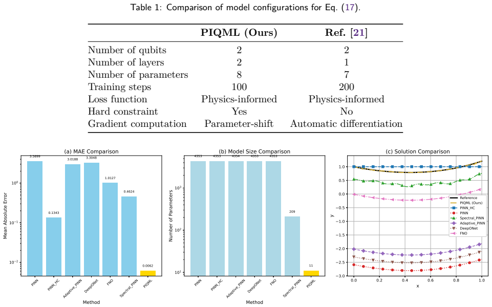
- [Section 3.1, Table 1 and baseline comparison] The model configuration is reported inconsistently. Table 1 states that the PIQML model for Eq. (17) uses 2 qubits, 2 layers, and 8 parameters, while the baseline comparison paragraph immediately following states that the same model uses 11 total parameters. For a 2-qubit, 2-layer ansatz with three Euler rotations per qubit per layer, the ansatz alone has 3NL=12 parameters, so neither number is consistent with the stated architecture. This inconsistency affects the claimed resource efficiency and the comparison with classical baselines.
- [Section 3.4, Fig. 11] Panel (d) is labeled 'Differential Equation Residual' and panel (b) compares derivatives, but both rely on the derivative computed via the erroneous Eq. (13). Therefore the low residual and the derivative agreement shown in these panels are not evidence that the learned solution satisfies Eq. (22). Without a corrected residual, the nonlinear benchmark does not substantiate the paper's central claim.
minor comments (4)
- [Section 2.4.2, Eq. (13)] The notation in Eq. (13) is ambiguous: φ(x) appears both as a scalar argument and in the subscript Ûφ, and it is unclear whether the shift is applied to a single angle or to each qubit's angle independently. Clarifying this would help readers see the need for the chain-rule factors.
- [Section 2.1.1, Eq. (3)] The decomposition in Eq. (3) contains a typographical inconsistency in the subscript of the second term: it should be consistent with the quantum logic notation used elsewhere, and the relationship between n[j] on the left and n on the right should be defined explicitly.
- [Figure 11 caption] The caption and the main text describe the subfigures in different orders. The text lists (a) function value, (b) derivative, (c) absolute error, (d) residual, (e) training loss, (f) relative error, whereas the caption says (c) and (d) quantify absolute and relative errors and (e) visualizes the residual. The caption should match the panel labels.
- [References] Reference [21] is a GitHub repository rather than a peer-reviewed source; the comparison baseline would be better supported by a published description of the method. Similarly, reference [32] is a software documentation page.
Circularity Check
The 'close agreement' with the benchmark is a training fit: y_cla is minimized by L_data and then reused as the ground truth, while the residual term that could break the loop does not enforce the ODE as written.
-
fitted input called prediction
[Section 2.5, Eq. (16); Section 3.4, Fig. 11(a)-(f)]
"L(i)_data(Θ) = [~y(x)−y_cla(x)]^2, where y_cla(x) denotes the classical numerical or analytical reference solution used to guide the quantum model toward physically meaningful solutions. ... The classical numerical reference solution is obtained using the Runge–Kutta method ... which serves as the ground truth for evaluating the quantum model’s accuracy."
The same classical solution y_cla is minimized by L_data during training and then reused as the evaluation benchmark in Fig. 11. Minimizing [~y−y_cla]^2 directly drives the model output to the reference, so the reported 'close agreement', absolute error, and relative error are training-fit comparisons, not independent predictions. The residual loss L_res is the only term that could break this circularity, but Eq. (13) omits the chain-rule factor dφ/dx for the Fourier and Chebyshev feature maps, so L_res does not actually enforce the stated differential equation; the central 'intrinsic satisfaction' claim is therefore not independently supported.
-
other
[Section 2.4.2, Eq. (13); Section 2.5, Eq. (15)]
"∂f(θ,x)/∂x = 1/2 [ f(Û_φ(φ(x)+π/2)) − f(Û_φ(φ(x)−π/2)) ] ... L(i)_res(Θ) = [ d~y(x)/dx − g(x,~y(x)) ]^2"
For the feature maps used here, φ_j(x)=2πω_j x and φ_j(x)=2n[j] arccos x, the parameter-shift rule gives the derivative with respect to the gate angle φ, not with respect to x; the correct chain-rule factors, 2πω_j and −2n[j]/√(1−x^2) summed over j, are absent. Consequently L_res as implemented is not the residual of the ODE dy/dx = g(x,y), so the abstract's claim that the model 'intrinsically satisfies the physical constraint' is not supported. With the physics term void, the reported agreement with y_cla is exactly what L_data enforced, making the benchmark agreement a circular validation rather than an independent test.
full rationale
Most of the construction is not circular: the hard-constraint trial solution Eq. (9), the kernel choices, the ansatz, and the general loss decomposition do not assume the target solution, and no load-bearing claim rests on a self-citation; refs [21] and [32] are external baselines. The circularity lies in the validation logic. Eq. (16) places y_cla into the training objective, and the same y_cla is subsequently used as the 'ground truth' for the error and agreement figures; the reported match is therefore a measure of training fit. The independent physics term L_res would rescue the evaluation, but Eq. (13) computes the parameter-shift with respect to φ without the chain-rule factor dφ/dx for the Fourier and Chebyshev encodings, so L_res is not the actual ODE residual. Consequently the claim that the model 'intrinsically satisfies the physical constraint' is not established independently of the supervised fit, and the benchmark agreement reduces to a data-fitting comparison.
Assumptions & free parameters
free parameters (8)
- Ansatz parameters theta =
e.g., 8, 11, 12, 32, or 48 parameters depending on problem; exact values inconsistent in text
- Output weights w and bias b =
not specified
- Fourier frequencies omega_j =
not specified
- Chebyshev degrees n[j] =
not specified
- Kernel choice K(x) =
linear or exponential
- Loss weights lambda_res and lambda_data =
not specified
- Collocation points M and sampling distribution =
not specified
- Optimizer hyperparameters =
not specified
assumptions (5)
- ad hoc to paper The parameter-shift rule gives the derivative of the circuit output with respect to the input x directly, as written in Eq. (13).
- domain assumption The trial solution y~=A+K(x)f(theta,x) can represent the exact solution over the whole domain with the chosen small PQC ansatz.
- domain assumption The RK45 classical reference y_cla used in L_data is sufficiently accurate to serve as ground truth.
- standard math The tested first-order ODEs with new initial conditions have unique solutions on [a,b].
- domain assumption The chosen feature maps provide enough expressivity for high-frequency targets such as sin(50x).
Cite this review
Pith. "Pith review of Physics-Informed Quantum Machine Learning with Hard Constraint Embedding for Nonlinear Differential Equations of the First Order." pith.science (2026). https://pith.science/paper/3TF7LOFC
@misc{pith2026260803029,
  author       = {Pith},
  title        = {Pith review of: Physics-Informed Quantum Machine Learning with Hard Constraint Embedding for Nonlinear Differential Equations of the First Order},
  year         = {2026},
  howpublished = {\url{https://pith.science/paper/3TF7LOFC}},
  note         = {Machine review of arXiv:2608.03029}
}
read the original abstract
Quantum algorithms based on linear-system approaches for solving differential equations demand qubit and precision resources beyond near-term capabilities. To address these challenges, this work proposes a physics-informed quantum machine learning (PIQML) framework with hard constraint embedding, specifically designed for NISQ era. Within this framework, parameterized quantum circuits serve as machine learning models, where the input variable is encoded into a high-dimensional feature space via a Fourier feature map. Subsequently, to eliminate approximation errors in critical physical conditions, the solution is constructed through a rigorously designed function mapper that analytically enforces initial conditions as hard constraints. Crucially, we compute derivatives with respect to the input variable using the parameter-shift rule---a quantum native gradient evaluation technique that avoids classical discretization. Unlike generic loss functions that target abstract data patterns, our loss function focuses on the differential equation residual and reference data. This design ensures that the trained model not only approximates the data but also intrinsically satisfies the physical constraint expressed by the DE itself. Our method is validated on several differential equations, including highly oscillatory ones, demonstrating its capability to tackle challenging nonlinear dynamics. Results demonstrate that our quantum model successfully learns the solution, showing close agreement with a high-precision classical numerical benchmark.
Figures


Figures from the paper (6 more)



Reference graph
Works this paper leans on
-
[1]
Quan- tum computation and quantum information
Michael A Nielsen and Isaac L Chuang. Quan- tum computation and quantum information . Cambridge university press, 2010. ISBN 9781107002173
work page 2010
-
[2]
AHMAD Najmuddin and CHARAN Shiv. Study of stability criteria of numerical solution of or- dinary and partial differential equations using eulers and finite difference scheme. JOURNAL OF PARTIAL DIFFERENTIAL EQUATIONS , 35(3):281–288, 2022
work page 2022
-
[3]
Spec- tral element method in time for rapidly actuated systems
Mohammad H Kurdi and Philip S Beran. Spec- tral element method in time for rapidly actuated systems. Journal of Computational Physics , 227 (3):1809–1835, 2008
work page 2008
-
[4]
Quantum algorithm and circuit design solving the poisson equation
Yudong Cao, Anargyros Papageorgiou, Iasonas Petras, Joseph Traub, and Sabre Kais. Quantum algorithm and circuit design solving the poisson equation. New Journal of Physics , 15(1):013021, 2013
work page 2013
-
[5]
High-order quantum algo- rithm for solving linear differential equations
Dominic W Berry. High-order quantum algo- rithm for solving linear differential equations. Journal of Physics A: Mathematical and Theo- retical, 47(10):105301, 2014
work page 2014
-
[6]
Dominic W Berry, Andrew M Childs, Aaron Os- trander, and Guoming Wang. Quantum algo- rithm for linear differential equations with ex- ponentially improved dependence on precision. Communications in Mathematical Physics , 356 (3):1057–1081, 2017
work page 2017
-
[7]
Quan- tum spectral methods for differential equations
Andrew M Childs and Jin-Peng Liu. Quan- tum spectral methods for differential equations. Communications in Mathematical Physics , 375 (2):1427–1457, 2020
work page 2020
-
[8]
Quantum computing in the nisq era and beyond
John Preskill. Quantum computing in the nisq era and beyond. Quantum, 2:79, 2018
2018
Show all 34 references
-
[9]
Parameterized quantum circuits as machine learning models
Marcello Benedetti, Erika Lloyd, Stefan Sack, and Mattia Fiorentini. Parameterized quantum circuits as machine learning models. Quantum science and technology , 4(4):043001, 2019
2019
-
[10]
The theory of variational hybrid quantum-classical algorithms
Jarrod R McClean, Jonathan Romero, Ryan Babbush, and Alán Aspuru-Guzik. The theory of variational hybrid quantum-classical algorithms. New Journal of Physics , 18(2):023023, 2016
2016
-
[11]
Hardware- efficient variational quantum eigensolver for small molecules and quantum magnets
Abhinav Kandala, Antonio Mezzacapo, Kristan Temme, Maika Takita, Markus Brink, Jerry M Chow, and Jay M Gambetta. Hardware- efficient variational quantum eigensolver for small molecules and quantum magnets. nature, 549(7671):242–246, 2017
2017
-
[12]
Quantum approximate op- timization algorithm for maxcut: A fermionic view
Zhihui Wang, Stuart Hadfield, Zhang Jiang, and Eleanor G Rieffel. Quantum approximate op- timization algorithm for maxcut: A fermionic view. Physical Review A , 97(2):022304, 2018
2018
-
[13]
Variational quantum linear solver
Carlos Bravo-Prieto, Ryan LaRose, Marco Cerezo, Yigit Subasi, Lukasz Cincio, and Patrick J Coles. Variational quantum linear solver. Quantum, 7:1188, 2023
2023
-
[14]
Quantum algo- rithms for feedforward neural networks
Jonathan Allcock, Chang-Yu Hsieh, Iordanis Kerenidis, and Shengyu Zhang. Quantum algo- rithms for feedforward neural networks. ACM Transactions on Quantum Computing, 1(1):1–24, 2020
2020
-
[15]
A quantum approximate optimization al- gorithm
Edward Farhi, Jeffrey Goldstone, and Sam Gut- mann. A quantum approximate optimization al- gorithm. arXiv preprint arXiv:1411.4028 , 2014
2014 arXiv
-
[16]
A variational quantum algorithm for the poisson equation based on the banded toeplitz systems
Xiaoqi Liu, Yuedi Qu, Ming Li, and Shu- Qian Shen. A variational quantum algorithm for the poisson equation based on the banded toeplitz systems. Communications in Theoreti- cal Physics , 77(4):045101, 2025
2025
-
[17]
Variational quantum algorithm based on the minimum po- tential energy for solving the poisson equation
Yuki Sato, Ruho Kondo, Satoshi Koide, Hideki Takamatsu, and Nobuyuki Imoto. Variational quantum algorithm based on the minimum po- tential energy for solving the poisson equation. Physical Review A , 104:052409, 2021
2021
-
[18]
Variational quantum evolution equation solver
Fong Yew Leong, Wei-Bin Ewe, and Dax Enshan Koh. Variational quantum evolution equation solver. Scientific reports, 12(1):10817, 2022
2022
-
[19]
Physics-informed neural networks: A deep learning framework for solving forward and inverse problems involving nonlinear partial differential equations
Maziar Raissi, Paris Perdikaris, and George E Karniadakis. Physics-informed neural networks: A deep learning framework for solving forward and inverse problems involving nonlinear partial differential equations. Journal of Computational physics, 378:686–707, 2019
2019
-
[20]
Physics-informed neural networks (pinns) for fluid mechanics: A review
Shengze Cai, Zhiping Mao, Zhicheng Wang, Minglang Yin, and George Em Karniadakis. Physics-informed neural networks (pinns) for fluid mechanics: A review. Acta Mechanica Sinica, 37(12):1727–1738, 2021
2021
-
[21]
T. Tsao. Quantum circuit for solving dif- ferential equation. GitHub repository,
-
[22]
Self-adaptive physics-informed quantum machine learning for solving differential equa- tions
Abhishek Setty, Rasul Abdusalamov, and Felix Motzoi. Self-adaptive physics-informed quantum machine learning for solving differential equa- tions. Machine Learning: Science and Technol- ogy, 6(1):015002, 2025
2025
-
[23]
Quantum physics-informed neural networks
Corey Trahan, Mark Loveland, and Samuel Dent. Quantum physics-informed neural networks. En- tropy, 26(8):649, 2024
2024
-
[24]
Hybrid quantum physics- informed neural networks for simulating compu- 11 tational fluid dynamics in complex shapes
Alexandr Sedykh et al. Hybrid quantum physics- informed neural networks for simulating compu- 11 tational fluid dynamics in complex shapes. Ma- chine Learning: Science and Technology , 5(2): 025045, 2024
2024
-
[25]
Solving transport equations on quantum computers—potential and limitations of physics-informed quantum circuits
Pia Siegl et al. Solving transport equations on quantum computers—potential and limitations of physics-informed quantum circuits. CEAS Aeronautical Journal, 16(1):63–80, 2025
2025
-
[26]
On physics-informed neural networks for quantum computers
Stefano Markidis. On physics-informed neural networks for quantum computers. Frontiers in Applied Mathematics and Statistics , 8:1036711, 2022
2022
-
[27]
Solving differential equations via continuous- variable quantum computers
Manik Knudsen and Christian B Mendl. Solving differential equations via continuous- variable quantum computers. arXiv preprint arXiv:2012.12220, 2020
2012 arXiv
-
[28]
Quantum physics-informed neural net- works for multivariable partial differential equa- tions
Giorgio Panichi, Sebastiano Corli, and Enrico Prati. Quantum physics-informed neural net- works for multivariable partial differential equa- tions. Physical Review Applied , 25(1):014001, 2026
2026
-
[29]
Physics-informed quantum machine learning: Solving nonlinear differential equations in latent spaces without costly grid evaluations
Annie E Paine, Vincent E Elfving, and Oleksandr Kyriienko. Physics-informed quantum machine learning: Solving nonlinear differential equations in latent spaces without costly grid evaluations. arXiv preprint arXiv:2308.01827 , 2023
2023 arXiv
-
[30]
Approximation Theory and Approximation Practice
Lloyd N Trefethen. Approximation Theory and Approximation Practice. SIAM, Philadelphia, ex- tended edition, 2019
2019
-
[31]
Eval- uating analytic gradients on quantum hardware
Maria Schuld, Ville Bergholm, Christian Gogolin, Josh Izaac, and Nathan Killoran. Eval- uating analytic gradients on quantum hardware. Physical Review A , 99(3):032331, 2019
2019
-
[32]
Qadence: A python package for differen- tiable digital-analog quantum programs
Pasqal. Qadence: A python package for differen- tiable digital-analog quantum programs. https: //pasqal-io.github.io/qadence/v1.5.2/,
-
[2022]
URL https://github.com/tytsao/ quantum-circuit-for-solving-differential-equation
-
[2024]
URL https://pasqal-io.github.io/ qadence/v1.5.2/. 12
Reviewed August 8, 2026 · model on record in the stance chip above.
Discussion (0). Continue with ORCID to comment.