REVIEW 4 major objections 8 minor 69 references
Voronoi Histograms for Adaptive Vectorization of Expected Persistence Diagrams
T0 review · 4 major / 8 minor · reviewed 2026-07-30 · grok-4.5
Pith's one-line read Expected Persistence Diagrams can be vectorized by counting mass in data-dependent Voronoi cells instead of smoothing each feature with a fixed kernel.
desk verdict Solid EPD tooling with an honest coarse-vs-smooth trade-off, but the Lipschitz stability theorem does not actually cover the atomic histograms used in the experiments. read the letter →
The pith
A machine-rendered reading of the paper's core claim, the machinery that carries it, and where it could break.
The reading
What carries the argument
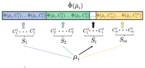
Vrep (Voronoi-based Representation): Φ(μ̄, C) = [μ̄(V(c₁)), …, μ̄(V(c_k))], the histogram of normalized EPD mass over Voronoi cells of a codebook C, concatenated over many sampled codebooks (Vrepd adds a diagonal cell). It carries the argument by replacing smooth functional summaries with adaptive partition-based mass counts, enabling the stability and conditional Wasserstein bounds.
What would settle it
Build synthetic EPD pairs whose Wasserstein gap is pure coarse mass shift across well-separated regions with small codebook approximation error: if Vrep’s ℓ₁ distances fail to track W₁ better than PI/PS/PL there—or if tasks that depend on total feature mass lose accuracy under the paper’s unit-mass normalization—the central trade-off claim does not hold.
Extended reading notes
Core claim
A Voronoi histogram of a normalized empirical Expected Persistence Diagram—mass counts inside cells of randomly sampled codebooks, concatenated across codebooks—is a stable finite vectorization that needs no explicit smooth point-transformation model, and under stated separation conditions it can preserve Wasserstein-scale differences at the cell level while matching or beating common smooth EPD summaries on topology-rich data.
Load-bearing premise
Every EPD is normalized to unit total mass before analysis and representation, so any signal in the absolute number or total mass of topological features is thrown away.
Editorial extensions
If this is right
- When the useful signal is coarse mass allocation on the birth–death plane, adaptive Voronoi counts can replace fixed-kernel EPD vectorizations.
- With support subsampling, EPD vectorization cost need not grow with the number of sampled persistence diagrams.
- A diagonal Voronoi cell can separate near-diagonal noise from persistent features more stably than interior-only codebooks.
- The same unsupervised vectors can feed dimensionality reduction where labeled end-to-end point-cloud models cannot.
Reading between the lines
- Hard cell assignment will under-resolve tasks driven by fine within-cell shape; hybrid pipelines that keep a smooth local descriptor inside large cells are a natural next test.
- Re-attaching total mass or unnormalized counts as extra coordinates would check how much the unit-mass step is costing on density-sensitive problems.
- Learned or quantized codebooks under the same hard-histogram readout could tighten the Wasserstein lower bound when random support samples miss modes.
Signed reviews
Editorial analysis
A structured set of objections, weighed in public.
Referee Report
Summary. The paper proposes Vrep/Vrepd, a vectorization of empirical Expected Persistence Diagrams (EPDs). An empirical EPD (the average measure of n sampled PDs, ℓ1-normalized to unit mass) is represented by concatenating, over t codebooks of size k sampled from EPD supports, the histogram of EPD mass in each Voronoi cell; Vrepd adds a cell centered at the diagonal. The contributions are: (i) the representation itself; (ii) a stability analysis (Lemmas 4.3–4.4, Thm. 4.5: ‖Φ̂(μ̄)−Φ̂(μ̄′)‖₁ ≤ LΔ) and a conditional Wasserstein lower bound (Thm. 4.6) relating histogram distance to W1 separation minus codebook approximation error; (iii) experiments: Random-Forest classification on Protein, CAD (with two noise levels), and five time-series-derived point-cloud datasets, where Vrep/Vrepd report higher mean accuracy than PI/PS/PL on all datasets; ablations over codebook sampling schemes; scale-up tests showing near-constant cost in n; comparisons to PWGK/SWK (kernels win on several datasets at much higher runtime); an unsupervised t-SNE/CH study; and a synthetic W1-correlation study. The paper is unusually candid about non-dominance and limitations, and the normalization premise is explicitly disclosed.
Significance. If the claims hold, this is a useful, simple, and computationally attractive EPD vectorization: near-constant cost in the number of sampled PDs (Fig. 6b) is a genuine practical advantage over PI/PS/PL, and the data-dependent Voronoi partition is a sensible alternative bias to fixed smooth kernels. The empirical package is stronger than typical: codebook-choice ablations (Table 2), scale-up tests, honest non-dominance results against PWGK/SWK (App. F.2), a controlled synthetic W1-correlation study (App. F.7) that explicitly shows where PI is preferable, codebook-construction alternatives (App. F.8), and promised code. The candid limitation section (D.5) and the conditional reading of Thm. 4.6 are commendable. The weak half is the theory: as written, the stability theorem does not cover the atomic object used in every experiment, and Lemma 4.3's proof has concrete gaps. Fixing or rescoping this would make the paper a solid contribution.
major comments (4)
- [§4.2, Def. 4.2, Lemma 4.3, Thm. 4.5] Population/empirical mismatch in the stability results. Def. 4.2, Lemma 4.3 and Thm. 4.5 quantify over the population EPD μ̄ = lim_{n→∞}(1/n)Σμ_i, and Lemma 4.3's proof requires μ̄ to admit a Lipschitz density p (via [16]) perturbed by convolution with Gaussian noise. The deployed pipeline (§4.1, App. E.1) instead histograms an atomic empirical EPD (n=50 sampled PDs, support subsampled to |S_μ̄|=50). For an atomic measure, μ ↦ μ(V(c)) is not Lipschitz in W1: an atom of mass ~1/50 sitting ε from a Voronoi edge crosses it under an ε-perturbation, shifting ‖Φ‖₁ by ~2/50 regardless of how small ε is. Thus no deterministic Lipschitz-in-W1 bound covers the regime of Table 1 and Fig. 5, and Fig. 5 — the only stability evidence — is itself run in that uncovered regime and shows averages on one dataset only. Additionally, Lemma 4.3 is stated for arbitrary μ̄′ (via an optimal matching η), but the
- [App. C.1 (proof of Lemma 4.3)] Several specific gaps need repair: (a) the final equality Σ_j M·W1·Vol(V(c_j)) = M·W1 implicitly uses Σ_j Vol(V(c_j)) = 1, but the cells partition Ω′, so the sum is Vol(Ω′); the constant should be M·Vol(Ω′) (directionally harmless, but the stated constant is wrong). (b) The text asserts 'α and ϵ is dependent of each other' and then writes r = p∗q, which is valid only under independence — either assume independence or replace the convolution step. (c) 'W1(μ̄,μ̄′) = ≤ ∫q(z)‖z‖dz': only ≤ holds; W1 is an infimum over couplings. (d) Def. 4.2 uses Δ both as a deterministic radius bound (‖r̂_j − r_j‖ < Δ) and as a Gaussian random variable Δ ~ N(0,Σ); Gaussian noise is unbounded, so the hard bound fails almost surely. Each item is individually fixable, but together they require a careful rewrite of the perturbation model and the proof.
- [§4.1 normalization; App. D.4/D.5] All theory and the main experiments ℓ1-normalize EPDs to unit mass, discarding total feature count / total persistence mass and making Wasserstein (rather than OTp) applicable. The authors disclose this in App. D.4/D.5, which is appropriate, but no experiment quantifies the cost. Since the motivation (§2) explicitly invokes OTp for unequal-mass EPDs, a cheap ablation would substantially clarify when the premise is safe: e.g., augment Φ̂ with log μ̄(Ω) as an extra feature, or an unnormalized variant, on a dataset where class plausibly correlates with feature count. Without it, the 'Wasserstein-scale variation' framing applies to a geometry whose match to the tasks is asserted, not checked.
- [§5, Tables 1–2] Accuracies are means over 10 random splits on small datasets (BirdChicken n=40, Beef n=60, Protein n=99), with no standard deviations, confidence intervals, or paired tests reported, yet the text claims Vrep/Vrepd 'outperform PI, PS and PL over all the datasets.' Several margins look within plausible split noise (e.g., CAD0.01: 0.912 vs PI 0.911; CAD0.01/CAD0.05 vs PI at 0.900–0.911; Earthquakes vs PL). Please report per-split standard deviations and a paired significance test, mark which differences are significant, and soften the blanket claim where they are not. This is load-bearing for the main empirical claim, not a presentational nicety.
minor comments (8)
- [App. C.2 (proof of Lemma 4.4)] The proof invokes 'Theorem 5.1 and Remark 5.3 in [4]', but [4] is Beer, 'The Hausdorff metric and convergence in measure'; footnote 7's arXiv link (1103.4125) shows Reem [49] is intended. Also 'd_H(V(c_i), V(c_j)) ≤ Δ/γ' should be V(c′_i), and 'bounder area' → 'bounded area'.
- [App. C.5 vs App. D.3 (Thm. D.1)] d_min(C) is defined with ‖·‖₁ in App. C.5 but with ‖·‖₂ in the App. D.3 restatement of Thm. D.1 — align. In the C.5 proof, '‖Φ(ν̄,C)−Φ(ν̄,C)‖' appears three times where (μ̄,ν̄) is meant.
- [App. C.4 (proof of Thm. 4.6)] The transported mass in the designed plan is exactly ½‖Φ(μ̄,C)−Φ(ν̄,C)‖₁ (the ℓ1 norm double-counts excess and deficit), so the stated bound holds with factor-2 slack — worth a remark, or tighten. Also the phrase 'optimal partial transport metric W1' in the proof is a misnomer since masses are equal here.
- [Thm. 4.5 constant L] L = mt(M_max + kC_0^max) grows linearly with dataset size m; App. D.2 shows mt cancels in the normalized δ, but the raw bound is vacuous at realistic m. A sentence on the practical meaning (and in-principle estimability) of the constants M and C_0, both of which depend on the unknown EPD density, would help readers gauge the bound's content.
- [Lemma 4.4 statement] Main text says C_0 is 'determined by μ̄ and C'; the App. C.2 restatement says 'determined by μ̄' — align.
- [Citation/formatting] Bracketed citation numbers render without brackets throughout ('As pointed by 69', 'motivated by Lemma 2 in 25'). In App. D.3, 'Theorem 0.5' does not exist — presumably Thm. 4.6 is meant. 'V oronoi' appears with a spurious space throughout. Fig. 5 would benefit from error bars across the 450 EPDs.
- [App. D.1 (PI/PS comparison example)] The example assumes codebook size k very large to get ‖Φ(μ,C)−Φ(ν,C)‖₁ = 2W(μ,ν); please comment on how the conclusion degrades at the k values used in practice (k ≤ 20, App. E.1).
- [§3 / Def. 4.1] Since Persistence Bag-of-Words [68] is the closest histogram-style prior art, consider discussing it in §3 rather than only footnote 3, with one sentence on hard Voronoi vs GMM soft assignment. Also state near Def. 4.1 what §5 only says later: for a test EPD the concatenation uses codebooks sampled from training EPDs only.
Circularity Check
No significant circularity: Vrep is an independently defined histogram; stability/W1 bounds are conditional inequalities, not fits renamed as predictions.
full rationale
The paper defines Φ as normalized EPD mass in Voronoi cells of sampled codebooks (Def. 4.1), then proves Lipschitz stability under stated perturbation/normalization/codebook conditions (Lemmas 4.3–4.4, Thm 4.5) and a conditional W1 lower/upper bound via triangle inequality and a designed transport plan (Thm 4.6, App. C). Those bounds are mathematical consequences of the definitions plus external facts (e.g. Chazal–Divol density existence [16], Hausdorff stability of Voronoi cells [4], Divol–Lacombe quantization motivation [25]); they do not fit a target metric from the classification labels or redefine the claimed quantity as its own input. Empirical tables compare unsupervised vectors plus Random Forest against PI/PS/PL and kernels on external datasets; accuracies are not forced by construction from fitted constants. Modeling choices (l1 normalization, codebook sampling) are assumptions, not circular reductions. Correctness gaps about atomic vs density EPDs are outside circularity. No self-citation uniqueness chain or ansatz-smuggling from the same authors is load-bearing.
Assumptions & free parameters
free parameters (6)
- codebook size k =
CV over 2–20 (t fixed at 10)
- number of codebooks t =
10
- EPD support subsample size |S_μ̄| =
50
- codebook sampling scheme =
default in main table; ablation in Table 2
- PI/PS/PL and kernel bandwidths / resolutions =
PI 10×10; bandwidths in {1e-4..1e-1}; PL kmax in {2,4,6,8}; resolution 100
- number and size of sampled PDs forming each EPD =
n=50; dataset-specific subsample fractions
assumptions (7)
- domain assumption A persistence diagram is a finite atomic measure on the birth-death half-plane; empirical EPD is the average of sampled PD measures.
- ad hoc to paper After normalizing EPD total mass to 1, Wasserstein distance is the appropriate dissimilarity and equal-mass comparison is valid.
- domain assumption EPD densities exist and are Lipschitz (or C^k) on a bounded filtration window so measure perturbation controls cell-mass change.
- standard math Voronoi cells of perturbed codebooks have Hausdorff distance O(Δ) under minimum-separation and domain assumptions (Beer-type geometric stability).
- domain assumption Lemma 2 of Divol–Lacombe: Voronoi coefficients μ(V(ci)) optimally represent a measure among measures supported on codebook C in OTp.
- ad hoc to paper For the W1 lower bound to be informative, codebook approximation errors must be small relative to W1(μ̄,ν̄) (well-resolved codebooks).
- domain assumption Random-forest accuracy on selected topology-sensitive datasets is a valid proxy for representation quality.
invented entities (1)
-
Vrep / Vrepd (Voronoi-based EPD histogram representation)
independent evidence
Cite this review
Pith. "Pith review of Voronoi Histograms for Adaptive Vectorization of Expected Persistence Diagrams." pith.science (2026). https://pith.science/paper/3UEXI67P
@misc{pith2026260727126,
  author       = {Pith},
  title        = {Pith review of: Voronoi Histograms for Adaptive Vectorization of Expected Persistence Diagrams},
  year         = {2026},
  howpublished = {\url{https://pith.science/paper/3UEXI67P}},
  note         = {Machine review of arXiv:2607.27126}
}
read the original abstract
Persistence Diagram (PD) is known to capture point cloud topology effectively, but its computation has high time complexity. Expected Persistence Diagram (EPD) has been developed to reduce the time cost by studying the topology of multiple subsets of a point cloud and it serves as a distribution of topological features. Existing EPD vectorizations often rely on predefined point transformations, such as Gaussian or landscape functions. We study an alternative discretization based on Voronoi histograms, which trades smooth functional approximation for adaptive partition-based counting. We propose to use Voronoi Diagram-based histogram as the vectorization of EPD, without imposing an explicit smooth point transformation model. Under stated separation and normalization conditions, we establish stability bounds and characterize when the histogram representation preserves Wasserstein-scale variation. We demonstrate the effectiveness of our proposed representation on real-world datasets which have significant topological features for classification and dimensionality reduction tasks.
Figures


Figures from the paper (12 more)



Reference graph
Works this paper leans on
-
[16]
The density of expected persistence diagrams and its kernel based estimation
Frédéric Chazal and Vincent Divol. The density of expected persistence diagrams and its kernel based estimation. InProceedings of International Symposium on Computational Geometry, 2018
2018
-
[1]
Persistence images: A stable vector representation of persistent homology.Journal of Machine Learning Research, 18, 2017
Henry Adams, Tegan Emerson, Michael Kirby, Rachel Neville, Chris Peterson, Patrick Shipman, Sofya Chepushtanova, Eric Hanson, Francis Motta, and Lori Ziegelmeier. Persistence images: A stable vector representation of persistent homology.Journal of Machine Learning Research, 18, 2017
2017
-
[2]
Persistent homology for breast tumor classification using mammogram scans.Mathematics, 10(21):4039, 2022
Aras Asaad, Dashti Ali, Taban Majeed, and Rasber Rashid. Persistent homology for breast tumor classification using mammogram scans.Mathematics, 10(21):4039, 2022
2022
-
[3]
On the stability of persistent entropy and new summary functions for topological data analysis.Pattern Recognition, 107:107509, 2020
Nieves Atienza, Rocío González-Díaz, and Manuel Soriano-Trigueros. On the stability of persistent entropy and new summary functions for topological data analysis.Pattern Recognition, 107:107509, 2020
2020
-
[4]
The hausdorff metric and convergence in measure.Michigan Mathematical Journal, 20(4):63–64, 1974
Gerald A Beer. The hausdorff metric and convergence in measure.Michigan Mathematical Journal, 20(4):63–64, 1974
1974
-
[5]
Springer Science & Business Media, 2007
Ingwer Borg and Patrick JF Groenen.Modern multidimensional scaling: Theory and applications. Springer Science & Business Media, 2007
2007
-
[6]
Random forests.Machine Learning, 45:5–32, 2001
Leo Breiman. Random forests.Machine Learning, 45:5–32, 2001
2001
-
[7]
P. Bubenik. Statistical topological data analysis using persistence landscapes.Journal of Machine Learning Research, 16:77–102, 01 2015
2015
Show all 69 references
-
[8]
The persistence landscape and some of its properties.Topological Data Analysis, 2020
Peter Bubenik. The persistence landscape and some of its properties.Topological Data Analysis, 2020
2020
-
[9]
A persistence landscapes toolbox for topological statistics.Journal of Symbolic Computation, 78:91–114, 2017
Peter Bubenik and Paweł Dłotko. A persistence landscapes toolbox for topological statistics.Journal of Symbolic Computation, 78:91–114, 2017
2017
-
[10]
A dendrite method for cluster analysis.Communications in Statistics-theory and Methods, 3(1):1–27, 1974
Tadeusz Cali´nski and Jerzy Harabasz. A dendrite method for cluster analysis.Communications in Statistics-theory and Methods, 3(1):1–27, 1974
1974
-
[11]
Approximating persistent homology for large datasets.arXiv preprint arXiv:2204.09155, 2022
Yueqi Cao and Anthea Monod. Approximating persistent homology for large datasets.arXiv preprint arXiv:2204.09155, 2022
2022
-
[12]
Perslay: A neural network layer for persistence diagrams and new graph topological signatures.International Conference on Artificial Intelligence and Statistics, 2020
Mathieu Carrière, Frédéric Chazal, Yuichi Ike, Théo Lacombe, Martin Royer, and Yuhei Umeda. Perslay: A neural network layer for persistence diagrams and new graph topological signatures.International Conference on Artificial Intelligence and Statistics, 2020
2020
-
[13]
Sliced wasserstein kernel for persistence diagrams
Mathieu Carrière, Marco Cuturi, and Steve Oudot. Sliced wasserstein kernel for persistence diagrams. International Conference on Machine Learning, 2017
2017
-
[14]
John-Marc Chandonia, Lindsey Guan, Shiangyi Lin, Changhua Yu, Naomi K Fox, and Steven E Brenner. Scope: improvements to the structural classification of proteins–extended database to facilitate variant interpretation and machine learning.Nucleic Acids Research, 50(D1):D553–D559, 2022
2022
-
[15]
Pointnet: Deep learning on point sets for 3d classification and segmentation.IEEE Conference on Computer Vision and Pattern Recognition, 2017
R Qi Charles, Hao Su, Mo Kaichun, and Leonidas J Guibas. Pointnet: Deep learning on point sets for 3d classification and segmentation.IEEE Conference on Computer Vision and Pattern Recognition, 2017
2017
-
[17]
Subsampling methods for persistent homology.International Conference on Machine Learning, 2015
Frédéric Chazal, Brittany Fasy, Fabrizio Lecci, Bertrand Michel, Alessandro Rinaldo, and Larry Wasserman. Subsampling methods for persistent homology.International Conference on Machine Learning, 2015
2015
-
[18]
Stochas- tic convergence of persistence landscapes and silhouettes
Frédéric Chazal, Brittany Terese Fasy, Fabrizio Lecci, Alessandro Rinaldo, and Larry Wasserman. Stochas- tic convergence of persistence landscapes and silhouettes. InProceedings of Annual Symposium on Computational Geometry, pages 474–483, 2014
2014
-
[19]
An introduction to topological data analysis: Fundamental and practical aspects for data scientists.Frontiers in Artificial Intelligence, 4:667963, 2021
Frédéric Chazal and Bertrand Michel. An introduction to topological data analysis: Fundamental and practical aspects for data scientists.Frontiers in Artificial Intelligence, 4:667963, 2021
2021
-
[20]
Persistence paths and signature features in topological data analysis.IEEE Transactions on Pattern Analysis and Machine Intelligence, 42(1):192–202, 2018
Ilya Chevyrev, Vidit Nanda, and Harald Oberhauser. Persistence paths and signature features in topological data analysis.IEEE Transactions on Pattern Analysis and Machine Intelligence, 42(1):192–202, 2018
2018
-
[21]
An entropy-based persistence barcode.Pattern Recognition, 48(2):391–401, 2015
Harish Chintakunta, Thanos Gentimis, Rocio Gonzalez-Diaz, Maria-Jose Jimenez, and Hamid Krim. An entropy-based persistence barcode.Pattern Recognition, 48(2):391–401, 2015
2015
-
[22]
Persistence curves: A canonical framework for summarizing persis- tence diagrams.Advances in Computational Mathematics, 48(1):6, 2022
Yu-Min Chung and Austin Lawson. Persistence curves: A canonical framework for summarizing persis- tence diagrams.Advances in Computational Mathematics, 48(1):6, 2022. 10
2022
-
[23]
The ucr time series archive.IEEE/CAA Journal of Automatica Sinica, 6(6):1293–1305, 2019
Hoang Anh Dau, Anthony Bagnall, Kaveh Kamgar, Chin-Chia Michael Yeh, Yan Zhu, Shaghayegh Gharghabi, Chotirat Ann Ratanamahatana, and Eamonn Keogh. The ucr time series archive.IEEE/CAA Journal of Automatica Sinica, 6(6):1293–1305, 2019
2019
-
[24]
Comparing persistence diagrams through complex vectors
Barbara Di Fabio and Massimo Ferri. Comparing persistence diagrams through complex vectors. InImage Analysis and Processing, pages 294–305. Springer, 2015
2015
-
[25]
Estimation and quantization of expected persistence diagrams.Interna- tional Conference On Machine Learning, 2021
Vincent Divol and Théo Lacombe. Estimation and quantization of expected persistence diagrams.Interna- tional Conference On Machine Learning, 2021
2021
-
[26]
Persistence b-spline grids: stable vector representation of persistence diagrams based on data fitting.Machine Learning, 113(3):1373–1420, 2024
Zhetong Dong, Hongwei Lin, Chi Zhou, Ben Zhang, and Gengchen Li. Persistence b-spline grids: stable vector representation of persistence diagrams based on data fitting.Machine Learning, 113(3):1373–1420, 2024
2024
-
[27]
Edelsbrunner, D
H. Edelsbrunner, D. Letscher, and A. Zomorodian. Topological persistence and simplification. In Proceedings of Annual Symposium on Foundations of Computer Science, 2000
2000
-
[28]
The union of balls and its dual shape
Herbert Edelsbrunner. The union of balls and its dual shape. InProceedings of Annual Symposium on Computational Geometry, pages 218–231, 1993
1993
-
[29]
Representing size functions by complex polynomials.Proc
Massimo Ferri and Claudia Landi. Representing size functions by complex polynomials.Proc. Math. Met. in Pattern Recognition, 9:16–19, 1999
1999
-
[30]
The optimal partial transport problem.Archive for Rational Mechanics and Analysis, 195(2):533–560, 2010
Alessio Figalli. The optimal partial transport problem.Archive for Rational Mechanics and Analysis, 195(2):533–560, 2010
2010
-
[31]
Scope: Structural classification of pro- teins—extended, integrating scop and astral data and classification of new structures.Nucleic Acids Research, 42(D1):D304–D309, 2014
Naomi K Fox, Steven E Brenner, and John-Marc Chandonia. Scope: Structural classification of pro- teins—extended, integrating scop and astral data and classification of new structures.Nucleic Acids Research, 42(D1):D304–D309, 2014
2014
-
[32]
On the vietoris-rips complexes and a cohomology theory for metric spaces
Jean-Claude Hausmann et al. On the vietoris-rips complexes and a cohomology theory for metric spaces. Annals of Mathematics Studies, 138:175–188, 1995
1995
-
[33]
Graph filtration learning.International Conference on Machine Learning, 2020
Christoph Hofer, Florian Graf, Bastian Rieck, Marc Niethammer, and Roland Kwitt. Graph filtration learning.International Conference on Machine Learning, 2020
2020
-
[34]
Deep learning with topological signatures.Advances in Neural Information Processing Systems, 2017
Christoph Hofer, Roland Kwitt, Marc Niethammer, and Andreas Uhl. Deep learning with topological signatures.Advances in Neural Information Processing Systems, 2017
2017
-
[35]
Hofer, Roland Kwitt, and Marc Niethammer
Christoph D. Hofer, Roland Kwitt, and Marc Niethammer. Learning representations of persistence barcodes. Journal of Machine Learning Research, 20(126):1–45, 2019
2019
-
[36]
Topological graph neural networks.International Conference on Learning Representations, 2021
Max Horn, Edward De Brouwer, Michael Moor, Yves Moreau, Bastian Rieck, and Karsten Borgwardt. Topological graph neural networks.International Conference on Learning Representations, 2021
2021
-
[37]
Tropical coordinates on the space of persistence barcodes.Foundations of Computational Mathematics, 19(1):101–129, 2019
Sara Kališnik. Tropical coordinates on the space of persistence barcodes.Foundations of Computational Mathematics, 19(1):101–129, 2019
2019
-
[38]
A large-scale annotated mechanical components benchmark for classification and retrieval tasks with deep neural networks
Sangpil Kim, Hyung gun Chi, Xiao Hu, Qixing Huang, and Karthik Ramani. A large-scale annotated mechanical components benchmark for classification and retrieval tasks with deep neural networks. European Conference on Computer Vision, 2020
2020
-
[39]
Kernel method for persistence diagrams via kernel embedding and weight factor.Journal of Machine Learning Research, 18(1):6947–6987, 2017
Genki Kusano, Kenji Fukumizu, and Yasuaki Hiraoka. Kernel method for persistence diagrams via kernel embedding and weight factor.Journal of Machine Learning Research, 18(1):6947–6987, 2017
2017
-
[40]
Persistence weighted gaussian kernel for topological data analysis.International Conference on Machine Learning, 2016
Genki Kusano, Yasuaki Hiraoka, and Kenji Fukumizu. Persistence weighted gaussian kernel for topological data analysis.International Conference on Machine Learning, 2016
2016
-
[41]
Persistence fisher kernel: A riemannian manifold kernel for persistence diagrams.Advances in Neural Information Processing Systems, 2018
Tam Le and Makoto Yamada. Persistence fisher kernel: A riemannian manifold kernel for persistence diagrams.Advances in Neural Information Processing Systems, 2018
2018
-
[42]
Quantifying similarity of pore-geometry in nanoporous materials.Nature Communications, 8(1):1–8, 2017
Yongjin Lee, Senja D Barthel, Paweł Dłotko, S Mohamad Moosavi, Kathryn Hess, and Berend Smit. Quantifying similarity of pore-geometry in nanoporous materials.Nature Communications, 8(1):1–8, 2017
2017
-
[43]
On the dynamics of discrete food chains: Low-and high-frequency behavior and optimality of chaos.Journal of Mathematical Biology, 45(5):396–418, 2002
Torsten Lindström. On the dynamics of discrete food chains: Low-and high-frequency behavior and optimality of chaos.Journal of Mathematical Biology, 45(5):396–418, 2002
2002
-
[44]
Dowker complex based machine learning (dcml) models for protein-ligand binding affinity prediction.PLOS Computational Biology, 18(4):1 – 17, 2022
Xiang Liu, Huitao Feng, Jie Wu, and Kelin Xia. Dowker complex based machine learning (dcml) models for protein-ligand binding affinity prediction.PLOS Computational Biology, 18(4):1 – 17, 2022. 11
2022
-
[45]
Weighted persistent homology for biomolecular data analysis.Scientific Reports, 10(1):1–15, 2020
Zhenyu Meng, D Vijay Anand, Yunpeng Lu, Jie Wu, and Kelin Xia. Weighted persistent homology for biomolecular data analysis.Scientific Reports, 10(1):1–15, 2020
2020
-
[46]
Adaptive topological feature via persistent homology: filtration learning for point clouds.Advances in Neural Information Processing Systems, 2024
Naoki Nishikawa, Yuichi Ike, and Kenji Yamanishi. Adaptive topological feature via persistent homology: filtration learning for point clouds.Advances in Neural Information Processing Systems, 2024
2024
-
[47]
Approximating continuous functions on persistence diagrams using template functions.Foundations of Computational Mathematics, 23(4):1215– 1272, 2023
Jose A Perea, Elizabeth Munch, and Firas A Khasawneh. Approximating continuous functions on persistence diagrams using template functions.Foundations of Computational Mathematics, 23(4):1215– 1272, 2023
2023
-
[48]
Luis Polanco and Jose A. Perea. Adaptive template systems: Data-driven feature selection for learning with persistence diagrams.International Conference On Machine Learning And Applications, 2019
2019
-
[49]
The geometric stability of voronoi diagrams with respect to small changes of the sites
Daniel Reem. The geometric stability of voronoi diagrams with respect to small changes of the sites. In Proceedings of Annual Symposium on Computational Geometry, pages 254–263, 2011
2011
-
[50]
A stable multi-scale kernel for topological machine learning.IEEE Conference on Computer Vision and Pattern Recognition, 2015
Jan Reininghaus, Stefan Huber, Ulrich Bauer, and Roland Kwitt. A stable multi-scale kernel for topological machine learning.IEEE Conference on Computer Vision and Pattern Recognition, 2015
2015
-
[51]
Gaussian mixture models.Encyclopedia of biometrics, 741(659-663), 2009
Douglas A Reynolds et al. Gaussian mixture models.Encyclopedia of biometrics, 741(659-663), 2009
2009
-
[52]
Atol: measure vectoriza- tion for automatic topologically-oriented learning
Martin Royer, Frédéric Chazal, Clément Levrard, Yuhei Umeda, and Yuichi Ike. Atol: measure vectoriza- tion for automatic topologically-oriented learning. InInternational Conference on Artificial Intelligence and Statistics, pages 1000–1008. PMLR, 2021
2021
-
[53]
Characterisation of the idiotypic immune network through persistent entropy.European Conference on Complex Systems, 2016
Matteo Rucco, Filippo Castiglione, Emanuela Merelli, and Marco Pettini. Characterisation of the idiotypic immune network through persistent entropy.European Conference on Complex Systems, 2016
2016
-
[54]
Simplicial complexes and complex systems
Vsevolod Salnikov, Daniele Cassese, and Renaud Lambiotte. Simplicial complexes and complex systems. European Journal of Physics, 40(1):014001, 2018
2018
-
[55]
On time-series topological data analysis: New data and opportunities.IEEE Conference on Computer Vision and Pattern Recognition workshops, 2016
Lee M Seversky, Shelby Davis, and Matthew Berger. On time-series topological data analysis: New data and opportunities.IEEE Conference on Computer Vision and Pattern Recognition workshops, 2016
2016
-
[56]
Support vector machine.Machine learning models and algorithms for big data classification: thinking with examples for effective learning, pages 207–235, 2016
Shan Suthaharan and Shan Suthaharan. Support vector machine.Machine learning models and algorithms for big data classification: thinking with examples for effective learning, pages 207–235, 2016
2016
-
[57]
Representation of molecular structures with persistent homology for machine learning applications in chemistry.Nature Communications, 11(1):1–9, 2020
Jacob Townsend, Cassie Putman Micucci, John H Hymel, Vasileios Maroulas, and Konstantinos D V ogiatzis. Representation of molecular structures with persistent homology for machine learning applications in chemistry.Nature Communications, 11(1):1–9, 2020
2020
-
[58]
Visualizing data using t-sne.Journal of Machine Learning Research, 9(11), 2008
Laurens Van der Maaten and Geoffrey Hinton. Visualizing data using t-sne.Journal of Machine Learning Research, 9(11), 2008
2008
-
[59]
Attention is all you need.Advances in Neural Information Processing Systems, 2017
A Vaswani. Attention is all you need.Advances in Neural Information Processing Systems, 2017
2017
-
[60]
The wasserstein distances.Optimal transport: old and new, pages 93–111, 2009
Cédric Villani. The wasserstein distances.Optimal transport: old and new, pages 93–111, 2009
2009
-
[61]
Multiset transformer: Advancing representation learning in persistence diagrams.arXiv preprint arXiv:2411.14662, 2024
Minghua Wang, Ziyun Huang, and Jinhui Xu. Multiset transformer: Advancing representation learning in persistence diagrams.arXiv preprint arXiv:2411.14662, 2024
2024 arXiv
-
[62]
Topological data analysis.Annual Review of Statistics and Its Application, 5:501–532, 2018
Larry Wasserman. Topological data analysis.Annual Review of Statistics and Its Application, 5:501–532, 2018
2018
-
[63]
On the estimation of persistence intensity functions and linear representations of persistence diagrams.International Conference on Artificial Intelligence and Statistics, 2024
Weichen Wu, Jisu Kim, and Alessandro Rinaldo. On the estimation of persistence intensity functions and linear representations of persistence diagrams.International Conference on Artificial Intelligence and Statistics, 2024
2024
-
[64]
Multiscale persistent functions for biomolecular structure characteri- zation.Bulletin of mathematical biology, 80:1–31, 2018
Kelin Xia, Zhiming Li, and Lin Mu. Multiscale persistent functions for biomolecular structure characteri- zation.Bulletin of mathematical biology, 80:1–31, 2018
2018
-
[65]
Multidimensional persistence in biomolecular data.Journal of Computational Chemistry, 36(20):1502–1520, 2015
Kelin Xia and Guo-Wei Wei. Multidimensional persistence in biomolecular data.Journal of Computational Chemistry, 36(20):1502–1520, 2015
2015
-
[66]
Deep sets.Advances in Neural Information Processing Systems, 2017
Manzil Zaheer, Satwik Kottur, Siamak Ravanbakhsh, Barnabas Poczos, Russ R Salakhutdinov, and Alexander J Smola. Deep sets.Advances in Neural Information Processing Systems, 2017
2017
-
[67]
Gefl: extended filtration learning for graph classifica- tion.Learning on Graphs Conference, 2022
Simon Zhang, Soham Mukherjee, and Tamal K Dey. Gefl: extended filtration learning for graph classifica- tion.Learning on Graphs Conference, 2022. 12
2022
-
[68]
Persistence bag-of-words for topological data analysis.International Joint Conference on Artificial Intelligence, 2019
Bartosz Zieli´nski, Michał Lipi´nski, Mateusz Juda, Matthias Zeppelzauer, and Paweł Dłotko. Persistence bag-of-words for topological data analysis.International Joint Conference on Artificial Intelligence, 2019
2019
-
[69]
Computing persistent homology
Afra Zomorodian and Gunnar Carlsson. Computing persistent homology. InProceedings of Annual Symposium on Computational Geometry, page 347–356, 2004. A Vectorization methods of PD Here we introduce unsupervised and supervised vectorization methods for PD. • For unsupervised met...
2004 arXiv
Reviewed July 30, 2026 · model on record in the stance chip above.
Discussion (0). Continue with ORCID to comment.