REVIEW 3 major objections 4 minor 19 references
Cosmological Perturbations from a New Approach to Inflation
T0 review · 3 major / 4 minor · reviewed 2026-08-10 · deepseek-v4-flash
Pith's one-line read A nearly static 'lingering' universe is unstable and naturally tips into inflation.
desk verdict The n=2 'inflation-like' solution is actually coasting; the paper's explicit example doesn't support its central claim, though the perturbation formalism is a useful start. read the letter →
The pith
A machine-rendered reading of the paper's core claim, the machinery that carries it, and where it could break.
The reading
What carries the argument
The central object is the curvature perturbation $\zeta$ and its associated canonical variable $u_n = (a/\kappa)\sqrt{2/D_n}\,\Phi_n$, with $z_n = (H/a)\sqrt{3/(2D_n)}$ and $D_n = H^2 - H' + 1$, which turns the metric perturbation equation into $u'' + (c_{s,T}^2 (k^2-1) - z''/z)u = 0$ on a 3-sphere, where spatial Laplacian eigenvalues are $-(k^2-1)$ for integer $k$. The sign of $c_{s,T}^2$ and the ratio $z''/z$ decide whether modes oscillate or grow; during exact lingering $z''/z$ becomes a constant, and during post-lingering the equation reduces to a Whittaker equation. This lets the authors connect initial conditions in the static phase to late-time $\zeta$ without solving the full two-fluid system.
What would settle it
Compute the full perturbation evolution on the exact quasi-lingering background with small but nonzero $H$ and $H'$, and compare the mode growth rates to the static-limit predictions; if thresholds such as $w_s > 1/11$ shift, the stability analysis would need revision. Observationally, the model is falsified by a precise detection of zero spatial curvature or by the absence of the transplanckian spectral features it predicts.
Extended reading notes
Core claim
The central claim is that the lingering universe is real as a dynamical possibility: for a closed FLRW background with two fluids (one matter-like, one with equation of state $w_e \le -1/3$), there is an exact static fixed point, and nearby trajectories spend a long time 'lingering' before accelerating into inflation. Perturbations around the exact static solution are unstable for large-scale modes: the $k=1$ mode grows exponentially for any matter equation of state, $k=2$ vanishes by isotropy, and higher modes oscillate only if the matter equation of state exceeds $1/(k^2+2)$ for the matter-plus-cosmological-constant case, or more generally if the effective total sound speed is positive. During the quasi-lingering phase the perturbation equation is an oscillator with time-dependent frequency set by $z''/z$; growth in lingering must be compensated by decay post-lingering, which the paper verifies numerically for matter+cosmological constant, radiation+cosmological constant, and radiation+string-network fluids. The curvature perturbation $\zeta$ can be computed across both phases, giving a route to observables.
Load-bearing premise
The stability conclusions are derived for a perfectly static background with $H = H' = 0$, but they are applied to the quasi-lingering phase where $H$ is small but nonzero; the paper does not quantify the error this approximation introduces.
Editorial extensions
If this is right
- If lingering is real, the universe's pre-inflationary phase can be nearly static with an almost infinite Hubble time, so the 'age' of the universe is not defined by a single clock.
- Perturbations generated during lingering grow; matching to CMB amplitudes requires a compensating decay after inflation, which constrains the duration of both lingering and inflation.
- The model predicts small positive spatial curvature (as hinted by Planck 2018) and sets a lower bound on inflation duration from curvature alone.
- Transplanckian effects could be observable because modes start sub-Hubble in a nearly static phase.
- Stability analysis shows the static phase is a saddle point, so no fine-tuning is required to exit into inflation.
Reading between the lines
- The static approximation's validity for small but nonzero $H$ is not quantified; testing exact quasi-lingering stability could change the conclusions.
- The $k=2$ dipole mode vanishing is an artifact of linear perturbations; nonlinear effects might revive it and affect the CMB.
- The same machinery could be extended to the string-theory dilaton realization to make predictions for the Hagedorn phase and its CMB signatures.
- Because $c_{s,T}^2$ can be negative during lingering, the model may produce non-Gaussianities or specific spectral features that distinguish it from standard slow-roll inflation.
Editorial analysis
A structured set of objections, weighed in public.
Referee Report
Summary. The paper studies cosmological perturbations in a closed FLRW universe with two fluids, one satisfying 0 ≤ n ≤ 2 (exotic fluid with we ≤ −1/3) and one satisfying m ≥ 3 (standard matter), following the "lingering universe" proposal of the authors' previous work. It analyzes an exact static solution in which the scale factor is constant, the quasi-lingering phase in which the scale factor slowly evolves away from that static solution, and the post-lingering phase. The perturbation equations are derived in the curvature eigenfunction basis, and stability is assessed for several fluid combinations. The paper claims that the lingering phase is classically unstable and that the universe transitions into inflation, and it presents numerical and analytic solutions for Φ, density contrasts, and ζ during lingering and post-lingering phases, with the stated goal of establishing observables for this new paradigm.
Significance. If the generic n<2 branch indeed leads to accelerated expansion and the perturbation evolution can be matched to CMB observations, the lingering-universe scenario would be a genuinely different alternative to eternal inflation and cyclic cosmologies, with possible implications for transplanckian physics and for the initial-singularity debate. The paper's strengths include the explicit analytic treatment of the background, the use of the correct curved-space eigenmode decomposition, and the derivation of closed-form and special-function solutions for the perturbation variable u. However, the paper does not deliver the promised observables: there is no power spectrum, no normalization, and no matching calculation to CMB amplitudes. More seriously, the principal explicit case n=2, which is used for the detailed perturbation analysis and figures, is a coasting solution rather than inflation, so the central claim of a transition to inflation is not demonstrated in the paper's most concrete calculable example.
major comments (3)
- [II.B and III.F] The n=2 post-lingering solution is not inflationary. In Eq. (20), a^2(η) = a_pl^2 exp(√Δ_e Δη_pl), but converting to cosmic time gives t = (2a_pl/√Δ_e)(exp(√Δ_e Δη_pl/2) − 1) and hence a(t) = a_pl + (√Δ_e/2)t, so the cosmic-time second derivative of a vanishes. This is a coasting (Milne-like) solution with we = −1/3, not accelerated expansion. The paper describes n=2 as "particularly special" in Sec. II.A and uses it for the explicit perturbation analysis of Sec. III.F and Fig. 2; those perturbations are therefore not perturbations during an inflationary phase. The text and the Fig. 2 caption should be corrected to state that the exponential growth is only in conformal time, and the relevance of the n=2 perturbation results to CMB observables needs to be revisited or explicitly qualified.
- [III.C and III.D] Stability conclusions for the quasi-lingering phase are drawn from exact static perturbation equations in Sec. III.C (H = H′ = 0), but the quasi-lingering phase has small but nonzero H, as acknowledged in Sec. III.D. The paper does not quantify the error introduced by setting H = H′ = 0. Since quantities such as D_n and z_n in Sec. III.E depend on Δ_e and on the growing scale-factor deviation Δ(η), the static approximation should be justified by an explicit expansion in Δ_e or in H; otherwise the mode-by-mode stability statement, including the threshold condition (92), is not controlled.
- [I and III.F-H] The abstract and Introduction state that the goal is to establish observables and that any growth of perturbations in the lingering phase must be compensated by decay after lingering. However, the paper computes no power spectrum and performs no matching to CMB amplitudes; the plotted quantities (e.g., Φ and ζ in Figs. 2, 10, and 13) are evolved from arbitrary initial conditions. Moreover, in the n=2 case of Sec. III.F the post-lingering phase is explicitly found to be unstable for all k (A_pl^2 = we(k^2−1) − Δ_e < 0), which is growth, not the compensating decay required by the paper's own logic. The manuscript therefore does not yet establish an observable prediction of the lingering scenario in any calculable case.
minor comments (4)
- [Abstract and I] There are several typos: "transplackian" should be "transplanckian", "particularity" should be "particularly", and "ansätz" should be "ansatz".
- [III.G, Eq. (93)] The Mathieu functions MathieuC and MathieuS are introduced without defining their argument conventions; please specify the conventions used or provide a reference, since the parameters are nonstandard.
- [III.C] The sentence "The k = 2 mode vanishes in the linear perturbation theory by the background assumption of isotropy (the dipole vanishes)" is confusing: in the curvature eigenfunction labeling, k = 1 is the lowest nontrivial mode and k = 2 is not the dipole. Please clarify which mode is being discussed and why isotropy removes it.
- [II.B, Eq. (20)] Equation (20) introduces a_pl without defining it explicitly; it should be defined as the scale factor at the start of the post-lingering phase, and the notation Δη_pl should be defined consistently with Δη in Sec. II.A.
Circularity Check
No significant circularity: the perturbation evolution is derived by integrating stated background equations, and the self-citation of the lingering background from [1] is not used to define the perturbation predictions.
full rationale
The perturbation derivation is self-contained: Eqs. (21)-(25) are the standard Mukhanov-Feldman-Brandenberger equations in Newtonian gauge; the curved-space eigenmode replacement ∇²→-(k²-1) follows external references [11-13]; and the background coefficients in Sec. IIIE are obtained by direct integration of the two-fluid Friedmann equations, not by fitting the perturbation output. The stability thresholds in Sec. IIIC and the n=2 solutions (89)-(91) are algebraic consequences of those equations. No CMB amplitude is fitted and then re-predicted; the paper only states in the Introduction that growth in lingering 'must be compensated' by later decay, without using CMB normalization to set parameters. The principal self-citation is the importation of the lingering fixed point and its hyperbolic instability from [1]: 'we remind the reader that it was from the phase space analysis in [1] that the lingering point is a hyperbolic fixed point that leads asymptotically to inflation' (Sec. IIA). This is a genuine self-citation and the background paradigm rests on it, but the paper's new perturbation calculation is not equivalent to [1] nor to any fitted observable, so the derivation chain does not close on itself. The n=2 post-lingering solution a²(η)=a_pl² exp(Δη_pl√Δ_e) (Eq. 20) giving a∝t in cosmic time is a substantive physical concern about whether the highlighted case is inflationary, but that is a correctness issue, not a circularity: Eq. (20) follows from the stated Friedmann equations rather than from the conclusion it is used to support. Overall, no significant circularity is present; the score of 2 reflects the minor, non-reductive self-citation of the background paradigm.
Assumptions & free parameters
free parameters (4)
- Delta_e (exotic fluid energy density deviation) =
10^-4 in numerical examples
- Initial perturbation amplitudes and phases =
u(0)=1, u'(0)=0; delta(0)=delta'(0)=10^-5 or 0.001; Phi(0)=2000, Phi'(0)=10^4
- Equation-of-state parameters m and n =
m=3,4; n=0,1,2 in cases
- Scale factor at lingering a_* =
Set by K=1 coordinate rescaling
assumptions (6)
- domain assumption Positive spatial curvature K=1 is required for the lingering phase
- domain assumption Existence and stability of the lingering fixed point derived in [1] (same authors)
- domain assumption Two-fluid system with 0<=n<=2, m>=3 and no NEC violation
- domain assumption No anisotropic stress, Newtonian gauge, adiabatic sound speed cs_i^2 = w_i
- domain assumption Initial homogeneous and isotropic patch is assumed
- standard math Linear perturbation theory on a closed S^3 background
invented entities (2)
-
Lingering phase (quasi-static universe)
-
Exotic fluid with we<=-1/3
Cite this review
Pith. "Pith review of Cosmological Perturbations from a New Approach to Inflation." pith.science (2026). https://pith.science/paper/4LCBEV64
@misc{pith2026250104669,
  author       = {Pith},
  title        = {Pith review of: Cosmological Perturbations from a New Approach to Inflation},
  year         = {2026},
  howpublished = {\url{https://pith.science/paper/4LCBEV64}},
  note         = {Machine review of arXiv:2501.04669}
}
read the original abstract
In a previous paper we proposed a new approach to the beginning of inflation -- a lingering universe. The universe begins in a lingering state with a nearly vanishing Hubble parameter. This calls into question the absolute age of the universe, as the Hubble time can be nearly infinite. It also provides promise for addressing the initial singularity of inflation and issues with quantum field theory in de Sitter space-time. Such models arise in classical cosmologies with non-vanishing spatial curvature (inspired by PLANCK 2018 data), and independently by models that arise in string cosmology. In this paper, we consider the importance of cosmological perturbations for the stability of the lingering phase and how this influences cosmological observations. Our goal is to establish observables in this new paradigm for the origin of inflation which is in contrast to eternal inflation and cyclic cosmologies. We also address questions of stability and the transition to inflation.
Figures


Figures from the paper (10 more)



Reference graph
Works this paper leans on
-
[1]
The evolution of the density contrast is given by Eq
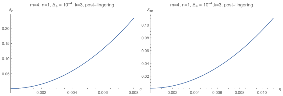
The curvature perturbationR ≈ −Φ during lingering. The evolution of the density contrast is given by Eq. 35 specialized to the case of a universe composed of matter and cosmological constant δ ′′ m + Hδ ′ m + (k2 − 1)Φ − 3HΦ ′ − 3Φ ′′ = 0, (95) there is no perturbation in a cc-like fluid. Fig. 4 shows the time evolution of the density contrast for k = 3 a...
-
[2]
Loitering Phase in Brane Gas Cosmology
R. Brandenberger, D. A. Easson, and D. Kimberly, Nucl. Phys. B 623, 421 (2002), arXiv:hep-th/0109165
work page Pith review arXiv 2002
-
[3]
Equation 69 for cosmological constant domination simplifies to Φ′′ + 3HΦ′ + 3H2 + 5 Φ = 0, (112) where we usedc2 s,T = 0 and wef f= −Ωe ∼ −(1 + ΩK) = − 1 + 1 H2 . (113) Eq. 112 corresponds to an underdamped harmonic oscillator. Figure 8 shows the evolu- tion of Φ assuming Φ(0) = 2000 and Φ′(0) = 104. Fig. 9 shows the time evolution of the density contrast...
-
[4]
B.Melcher, A.Pradhan, andS.Watson,Phys.Rev.D 110,063517(2024),arXiv:2310.06019 [hep-th]
arXiv 2024
-
[5]
S. Vagnozzi, A. Loeb, and M. Moresco, Astrophys. J. 908, 84 (2021), arXiv:2011.11645 [astro-ph.CO]
arXiv 2021
-
[6]
S. Vagnozzi, E. Di Valentino, S. Gariazzo, A. Melchiorri, O. Mena, and J. Silk, Phys. Dark Univ. 33, 100851 (2021), arXiv:2010.02230 [astro-ph.CO]
arXiv 2021
-
[7]
N. Aghanim et al. (Planck), Astron. Astrophys. 641, A6 (2020), [Erratum: As- tron.Astrophys. 652, C4 (2021)], arXiv:1807.06209 [astro-ph.CO]
arXiv 2020
- [8]
Show all 19 references
-
[9]
W. H. Kinney, S. Maity, and L. Sriramkumar, Phys. Rev. D 109, 043519 (2024), arXiv:2307.10958 [gr-qc]. 31
2024 arXiv
-
[10]
Borde, A
A. Borde, A. H. Guth, and A. Vilenkin, Phys. Rev. Lett. 90, 151301 (2003), arXiv:gr- qc/0110012
2003
-
[11]
D. A. Easson and J. E. Lesnefsky, (2024), arXiv:2404.03016 [hep-th]
2024 arXiv
-
[12]
Sahni, H
V. Sahni, H. Feldman, and A. Stebbins, Astrophys. J.385, 1 (1992)
1992
-
[13]
V. F. Mukhanov, H. Feldman, and R. H. Brandenberger, Phys. Rept.215, 203 (1992)
1992
-
[14]
E. M. Lifshitz and I. M. Khalatnikov, Adv. Phys.12, 185 (1963)
1963
-
[15]
N. D. Birrell and P. C. W. Davies,Quantum Fields in Curved Space, Cambridge Mono- graphs on Mathematical Physics (Cambridge Univ. Press, Cambridge, UK, 1984)
1984
-
[16]
Adams, N
A. Adams, N. Arkani-Hamed, S. Dubovsky, A. Nicolis, and R. Rattazzi, JHEP10, 014 (2006), arXiv:hep-th/0602178
2006 arXiv
-
[17]
Kaloper and S
N. Kaloper and S. Watson, Phys. Rev. D77, 066002 (2008), arXiv:0712.1820 [hep-th]
2008 arXiv
-
[18]
Geshnizjani, E
G. Geshnizjani, E. Ling, and J. Quintin, JHEP10, 182 (2023), arXiv:2305.01676 [gr-qc]
2023 arXiv
-
[19]
D. A. Easson and J. E. Lesnefsky, (2024), arXiv:2402.13031 [hep-th]. 32
2024
Reviewed August 10, 2026 · model on record in the stance chip above.
Discussion (0). Continue with ORCID to comment.