REVIEW 5 major objections 5 minor 37 references
Effects of Quantum Noise on Quantum Approximate Optimization Algorithm
T0 review · 5 major / 5 minor · reviewed 2026-08-14 · deepseek-v4-flash
Pith's one-line read Under common quantum noise channels, QAOA's output fidelity, cost function, and gradient all decay exponentially with circuit size and noise strength, while the parameter landscape is only rescaled, so optimized parameters do not shift.
desk verdict A QAOA noise study with solid numerical data and a worrying gap between the plotted exponentials and the 'noise only flattens' claim in the abstract. read the letter →
The pith
A machine-rendered reading of the paper's core claim, the machinery that carries it, and where it could break.
The reading
What carries the argument
The load-bearing object is the rescaling ansatz in Eq. (15): $f_{\mathrm{noise}}(\vec{\gamma},\vec{\beta})=(1-p)^{\alpha N} f_{\mathrm{ideal}}(\vec{\gamma},\vec{\beta}) + (1-(1-p)^{\alpha N})A$, with $A=0$ for the redefined Hamiltonian. The same exponential factor $ (1-p)^{\alpha N}$ is then carried linearly into the parameter-shift expressions for the gradient, making every partial derivative shrink by the same factor. The constant $\alpha$ is said to depend on the quantum circuit architecture and the noise model and is obtained by fitting simulation data rather than derived from the Kraus expansion.
What would settle it
Take a fixed QAOA instance and a fixed noise channel; measure the ratio $f_{\mathrm{noise}}(\vec{\gamma},\vec{\beta})/f_{\mathrm{ideal}}(\vec{\gamma},\vec{\beta})$ at many different parameter points, including points away from the optimum. If this ratio is not constant across the landscape, or if it departs from $(1-p)^{\alpha N}$ by more than sampling error, the claim that noise only rescales the parameter space is refuted. Equivalently, use a target Hamiltonian with $\mathrm{Tr}(H_p)\neq 0$ so $A\neq 0$ and optimize under noise: if the optimal parameters shift compared to the ideal run, the zero-$A$ assumption is doing load-bearing work.
Extended reading notes
Core claim
The paper's central claim is that the noisy cost function takes the form $f_{\mathrm{noise}}(\vec{\gamma},\vec{\beta})=(1-p)^{\alpha N} f_{\mathrm{ideal}}(\vec{\gamma},\vec{\beta})$ because the average cost term $A=\mathrm{Tr}(H_p)/2^m$ equals zero for the Max-Cut Hamiltonian $H_p=\sum_{i,j} C_{ij}Z_iZ_j$. It claims the same exponential factor rescales the cost-function gradient, and that output-state fidelity behaves as $F=(1-p)^{\delta N}$. Consequently, noise merely flattens the QAOA parameter space without changing its structure, so optimized parameters will not deviate from their ideal values. Numerical fits on a Max-Cut problem with QAOA step numbers $n=1$ through $4$ and noise strengths in $[0.0001,0.02]$ are presented as support.
Load-bearing premise
The formula $f_{\mathrm{noise}}=(1-p)^{\alpha N} f_{\mathrm{ideal}}$ with a single fitted exponent $\alpha$ and zero average term is assumed, not derived; if the actual scaling varies with the parameter or the constant $A$ is not negligible, the flat-landscape conclusion collapses.
Editorial extensions
If this is right
- QAOA parameter search can reuse noise-free optimized parameters on a noisy device, saving classical optimization cost.
- Larger QAOA layer number $n$ increases gate count $N$ and hence the noise decay $(1-p)^{\alpha N}$; beyond a noise-dependent depth, added layers stop helping.
- Gradient-based and gradient-free optimizers should follow approximately the same trajectory under noise, only slower.
- The same exponential decay implies output fidelity degrades predictably with circuit depth, enabling a pre-silicon noise budget for QAOA instances.
- The conclusion extends, as the paper notes, to multi-layer parameterized quantum circuits beyond QAOA.
Reading between the lines
- Beyond the paper: the same rescaling logic would predict that if a variational algorithm's Hamiltonian has a nonzero uniform average ($A\neq 0$), noise would shift the optimum rather than merely flatten it; that case is untested here.
- Beyond the paper: the fitted exponent $\alpha$ may itself grow with noise strength or depth in practice, which would make the simple $(1-p)^{\alpha N}$ law an approximation valid only at weak noise.
- Beyond the paper: a direct test on larger Max-Cut graphs or with correlated noise models would show whether a single fitted $\alpha$ remains universal enough to be predictive across problem sizes.
Editorial analysis
A structured set of objections, weighed in public.
Referee Report
Summary. The paper studies the effect of three quantum noise channels (dephasing, bit-flip, depolarizing) on the quantum approximate optimization algorithm (QAOA) applied to a 7-qubit Max-Cut instance. The central claims are that the output-state fidelity scales as (1-p)^(δN), the cost function scales as (1-p)^(αN) f_ideal, the gradient scales by the same factor, and as a consequence quantum noise merely flattens the QAOA parameter landscape without shifting the optimal parameters. These claims are supported by numerical simulations with a Monte-Carlo noisy quantum virtual machine, together with a statistical error analysis for the cost and gradient estimators.
Significance. If the central claim were rigorously established, the paper would provide a useful and simple characterization of noise resilience in QAOA, with practical implications for parameter optimization on NISQ devices. The numerical work and the statistical error analysis in Sec. V B are careful and are a genuine strength. However, the central scaling law is introduced as an ansatz rather than derived from the Kraus expansion, and the evidence is limited to a single parameter point and a single problem instance. As it stands, the paper offers a plausibility observation rather than a proven scaling theorem, and the strong conclusion that optimized parameters are unaffected by noise is not supported by the presented data.
major comments (5)
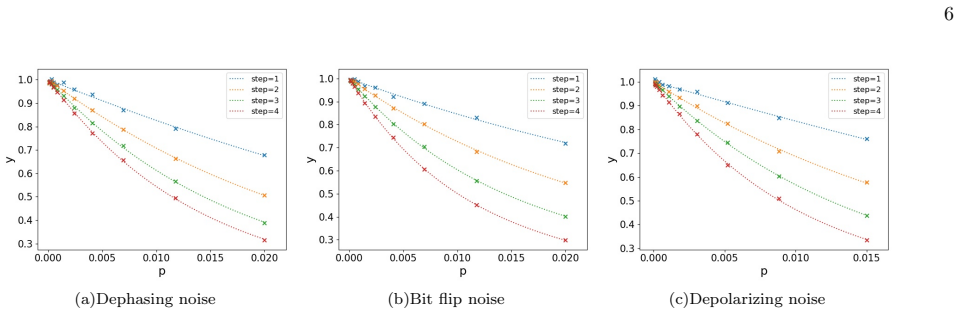
- [Sec. III B, Eq. (15)] The central scaling law f_noise = (1-p)^(αN) f_ideal is asserted, not derived. The text states that for small k the expectation of H_p is close to the ideal value and then "we use" the exponential form, with α a free constant. No derivation from the exact Kraus expansion in Eq. (14) is provided. Since Eq. (15) is the foundation for the gradient scaling in Eq. (18) and for the parameter-invariance conclusion in Sec. IV D, the main claim of the paper is currently an unproven ansatz.
- [Sec. III B, Eqs. (12)-(15)] The identification of A with the global average Tr(H_p)/2^m = 0 is unjustified. While H_p is traceless, the states |ψ_k⟩ in the noise expansion are not Haar-random states; they are obtained by applying a fixed set of Kraus operators to one particular product state. The weighted average of ⟨ψ_k|H_p|ψ_k⟩ over the large-k branches need not vanish, so the A=0 simplification can introduce a systematic error in the fitted scaling. This issue is load-bearing because if A is nonzero, Eq. (15) becomes a shift-plus-rescale rather than a pure flattening, and the conclusion that the optimum is unchanged would no longer follow.
- [Sec. IV B, Eqs. (19)-(20)] The exponent α is fitted from data at a single parameter setting, namely the ideal optimum. The paper does not test whether f_noise/f_ideal is constant across parameter space, which is exactly what Eq. (15) requires. Figures 4 and 5 only show the ratio at that one point. Without a parameter-space scan (e.g., random or grid-sampled γ,β) or an analytic derivation, the claim that noise merely rescales the whole landscape is unsupported.
- [Sec. IV D, Fig. 6] The optimization comparison is restricted to points satisfying Np<0.5, as stated in the caption. This restriction excludes the high-noise regime where the optimum would be most likely to shift if the simple rescaling picture breaks down. The text does not discuss this restriction or its implications, yet the conclusion that noisy optimized parameters equal ideal optimized parameters is based on this filtered data. The presented evidence is therefore insufficient for the strong claim made in the abstract and conclusion.
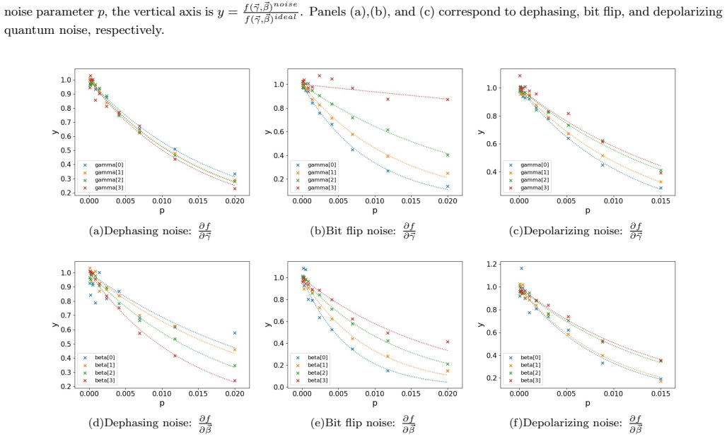
- [Sec. III C, Eq. (18)] The gradient scaling factor is inherited from the cost-function ansatz. However, the gradient formulas in Eqs. (16)-(17) involve cost functions evaluated at shifted parameters (γ_k ± π/2 and β_k ± π/2). Even if Eq. (15) held at the nominal point, it would need to hold at all shifted points for Eq. (18) to follow. This is not verified, and the assertion that α is nearly the same for different θ_k is made without numerical evidence in the manuscript.
minor comments (5)
- [Conclusion, Sec. V] The word "attens" appears in conclusion (1), which should read "flattens".
- [Introduction, Ref. [21]] "Sharma at al" should be "Sharma et al."
- [Fig. 5 caption] The caption states that panels (a) and (b) correspond to dephasing, (c) and (d) to bit-flip, and (e) and (f) to depolarizing noise, but the figure panels are arranged by derivative type (∂f/∂γ and ∂f/∂β) for each noise channel; the caption appears inconsistent with the panel labels.
- [Appendix B 1, Eq. (34)] The formula for L_costfunction contains a typographical artifact: "2 vuu√" should be a single square root symbol.
- [Sec. IV A] The statement that the fidelity data "fit well" with Eq. (9) is not quantified; reporting the fitted δ values and goodness-of-fit measures for all channels and steps would strengthen the presentation.
Circularity Check
The central noise-rescaling law is assumed in Eq. (15), its exponent α is fitted from the same data later shown as confirmation, and the gradient/optimization conclusions inherit that fitted factor.
-
other
[Sec. III B, Eq. (15)]
"We use (1−p)^{αN} f(γ,β)_ideal to represent the value of f(γ,β)_noise when k is small; here, α is a constant number. Therefore, the effect of the QAOA on the cost function is expressed as f(γ,β)_noise = (1−p)^{αN} f(γ,β)_ideal + (1−((1−p)^{αN})) A (15) in which A represents the average cost function of an arbitrary state. As shown before, A = Tr(Hp/2^m) = 0."
Eq. (15) is not obtained from the Kraus expansion in Eq. (14); it is an assumed exponential rescaling with a free parameter α. The step A = 0 uses the trace average of H_p over the whole Hilbert space, not the actual average over the noise-evolved branch states |ψ_k⟩, which all derive from one fixed input state. The parameter-independent form of the rescaling, which is the entire basis for the later conclusion that the landscape is only flattened, is therefore asserted rather than derived.
-
fitted input called prediction
[Sec. IV B, Eqs. (19)-(20)]
"We set the QAOA quantum circuit parameters choosing values corresponding to the ideal optimal parameter settings. ... We define y = f(γ,β)_noise / f(γ,β)_ideal (19), the relationship between y and noise parameter p being y = (1−p)^{αN}. (20) We fit the experimental test data with this formula; the fitted curves are drawn in Fig. 4."
The law claimed in Sec. III B, y = (1−p)^{αN}, is used verbatim as the fitting function, and α is extracted from the same numerical ratios that are then called a successful test. The fit is performed at the ideal optimal parameter setting only, a single point in parameter space. Fig. 4 therefore cannot establish that f_noise/f_ideal is constant across the whole parameter space; it only shows that a one-parameter exponential can be made to pass through data taken at one parameter point.
2 more flagged steps
-
fitted input called prediction
[Sec. III C Eq. (18) and Sec. IV C Eqs. (21)-(22)]
"the effect of quantum noise on the cost function gradient can then be written as ∂f(γ,β)/∂θ_k |_noise = (1−p)^{αn} ∂f(γ,β)/∂θ_k |_ideal (18) ... For Fig. 5, we have defined y = (∂f(γ,β)/∂θ_k)_noise / (∂f(γ,β)/∂θ_k)_ideal (21) and fitted the experimental data with the approximate formula y≈(1−p)^{αN}. (22)"
Eq. (18) is obtained by applying the scalar factor from Eq. (15) to every cost-function term that composes the gradient, so it inherits the fitted exponent α from the cost-function fit rather than providing new evidence. The numerical demonstration in Sec. IV C then fits the same exponential form y≈(1−p)^{αN} to the gradient ratios. Thus the gradient 'confirmation' is the same fitted input in new variables, and the conclusion that the parameter optimization path is unchanged is forced by the assumed scalar rescaling.
-
fitted input called prediction
[Sec. III A Eq. (9) and Sec. IV A]
"Considering this part of |φ_{i1,i2,...,iN}⟩, we infer the output state fidelity is expressed as F = (1−p)^{δN} (9), for which δ is a constant that depends on the quantum circuit architecture and quantum noise model. ... The numerical results are shown in Fig.2. It fits well with the Eq.(9)."
The exponential fidelity law is inferred rather than derived from the Kraus sum, and δ is then treated as an adjustable constant when comparing with numerical data in Fig. 2. This is the same fitted-ansatz pattern as the cost function. This step is peripheral to the parameter-optimization claim, but it shows that the paper's exponential scalings are curve fits to the data rather than parameter-free predictions.
full rationale
The central claim of the paper is Eq. (15): f_noise = (1−p)^{αN} f_ideal with one constant α and A = 0. This is introduced in Sec. III B as a representational ansatz, not derived from the Kraus expansion of Eq. (14). Sec. IV B then fits exactly this functional form to ratios measured at the ideal optimum and presents the fit (Fig. 4) as confirmation, which is tautological at the fitted point. Eq. (18) for the gradient is derived by inserting that same fitted scalar into every term, and Sec. IV C again fits y≈(1−p)^{αN} to gradient ratios, so the gradient and parameter-invariance conclusions inherit the fitted input. The fidelity law (9) follows the same fit-an-ansatz pattern. Because the claim that optimized parameters do not deviate requires the parameter-independent rescaling of Eq. (15) to hold everywhere, the paper's main assertion rests on a fitted input rather than an independent derivation. The A=0 step is also a logical gap: it uses the Hilbert-space trace average of H_p, not the average over the particular noise-evolved branch states generated from one fixed state. There is no load-bearing self-citation chain: refs. [30] and [31] are implementation/tool citations, not uniqueness or foundational support. The paper's own Fig. 6 test is restricted to points satisfying Np<0.5, so the high-noise regime where the scalar-rescaling assumption could fail is not tested. These limitations make the central claim partially circular (the predicted curve is the fitted curve) while the fidelity and gradient subsidiary laws are still empirical curve fits rather than independent predictions.
Assumptions & free parameters
free parameters (2)
- α (cost and gradient scaling exponent) =
not reported
- δ (state fidelity scaling exponent) =
not reported
assumptions (3)
- domain assumption Noise is modeled as a local Markovian channel applied after every gate, with Kraus operators of the form K={a0 I, a1 K1, ..., as Ks}.
- ad hoc to paper Only output branches with few errors contribute meaningfully; branches with many errors produce expectation values equal to the global average A=Tr(Hp)/2^m=0.
- ad hoc to paper The chosen 7-qubit Max-Cut graph with edge weights in Table I is representative of QAOA behavior for all problems.
Cite this review
Pith. "Pith review of Effects of Quantum Noise on Quantum Approximate Optimization Algorithm." pith.science (2026). https://pith.science/paper/4WDKZO65
@misc{pith2026190902196,
  author       = {Pith},
  title        = {Pith review of: Effects of Quantum Noise on Quantum Approximate Optimization Algorithm},
  year         = {2026},
  howpublished = {\url{https://pith.science/paper/4WDKZO65}},
  note         = {Machine review of arXiv:1909.02196}
}
read the original abstract
The quantum-classical hybrid algorithm is an algorithm that holds promise in demonstrating the quantum advantage in NISQ devices. When running such algorithms, effects from quantum noise are inevitable. In our work, we consider a well-known hybrid algorithm, the quantum approximate optimization algorithm (QAOA). We study the effects on QAOA from typical quantum noise channels and produce several numerical results. Our research indicates that the output state fidelity, the cost function, and its gradient obtained from QAOA decrease exponentially with respect to the number of gates and noise strength. Moreover, we find that noise merely flattens the parameter space without changing its structure, so optimized parameters will not deviate from their ideal values. Our result provides evidence for the effectiveness of hybrid algorithms running on NISQ devices.
Figures


Figures from the paper (4 more)


Reference graph
Works this paper leans on
-
[1]
Except for|φ0,0,...,0⟩, only a small part of|φi1,i2,...,iN⟩ has a value for|⟨φideal out |φi1,i2,...,iN⟩|2 that is significantly larger than 0. Considering this part of|φi1,i2,...,iN⟩, we infer the output state fidelity is expressed as F = (1−p)δN, (9) for which δ is a constant that depends on the quantum circuit architecture and quantum noise model. 3 B. Co...
-
[2]
In noisy quantum circuits, the quantum state is a mixed state and represented by a density matrix
Noisy Simulator First, we introduce the method of QPanda’s noisy QVM. In noisy quantum circuits, the quantum state is a mixed state and represented by a density matrix. In QPanda’s noisy QVM, we still use the state vector to rep- resent the quantum state and combine the Monte Carlo method to simulate mixed-state evolution under noisy quantum operations[32...
-
[3]
VQNet We use VQNet to realize QAOA. VQNet supports ideal and noisy QVM. The flow chart of QAOA is shown in Fig. 7. ⃗ γand ⃗β are QAOA quantum circuit parameters, “Variational Quantum Circuit” represents the QAOA quantum circuit, “Quantum Operator” is a basic oper- ator in VQNet, and the inputs of “Quantum Operator” are the “Variational Quantum Circuit” and...
-
[4]
The cost function is defined in Eq.(3)
Cost function statistical error To analyze cost function statistical error, we first in- troduce the method used to compute the cost function. The cost function is defined in Eq.(3). The method for calculating the expectation of Hp is as follows: First, Hp is decomposed into a sum of products of Pauli operators. Hp = ∑ i,j Hij, (27) where Hij =CijZiZj. Then...
-
[5]
Gradient Statistical Error The formulas of the derivatives of the cost function to parameters ⃗ γand ⃗β are presented in III C. They con- sist of some other cost functions, which were obtained by changing the QAOA quantum circuit parameter settings. Each cost function is a Gauss distribution and mutually independent. Therefore, the derivatives of the cost...
-
[6]
Preskill, Quantum 2, 79 (2018)
J. Preskill, Quantum 2, 79 (2018)
2018
-
[7]
Preskill, arXiv:1203.5813 [cond-mat, physics:quant-ph] (2012), arXiv: 1203.5813
J. Preskill, arXiv:1203.5813 [cond-mat, physics:quant-ph] (2012), arXiv: 1203.5813
arXiv 2012
-
[8]
C. Gidney and M. Eker, arXiv:1905.09749 [quant-ph] (2019), arXiv: 1905.09749
arXiv 2019
Show all 37 references
-
[9]
Mitarai, M
K. Mitarai, M. Negoro, M. Kitagawa, and K. Fujii, Phys- ical Review A 98, 032309 (2018)
2018
-
[10]
Havlek, A
V. Havlek, A. D. Crcoles, K. Temme, A. W. Harrow, A. Kandala, J. M. Chow, and J. M. Gambetta, Nature 567, 209 (2019)
2019
-
[11]
Lloyd and C
S. Lloyd and C. Weedbrook, Physical Review Letters 121, 040502 (2018)
2018
-
[12]
Dallaire-Demers and N
P.-L. Dallaire-Demers and N. Killoran, Physical Review A 98, 012324 (2018)
2018
-
[13]
Romero, J
J. Romero, J. P. Olson, and A. Aspuru-Guzik, Quantum Science and Technology 2, 045001 (2017)
2017
-
[14]
M. H. Amin, E. Andriyash, J. Rolfe, B. Kulchytskyy, and R. Melko, Physical Review X 8, 021050 (2018)
2018
- [15]
-
[16]
Schuld and N
M. Schuld and N. Killoran, arXiv:1803.07128 [quant-ph] (2018), arXiv: 1803.07128
2018 arXiv
-
[17]
Schuld, A
M. Schuld, A. Bocharov, K. Svore, and N. Wiebe, arXiv:1804.00633 [quant-ph] (2018), arXiv: 1804.00633
2018 arXiv
-
[18]
Schuld, M
M. Schuld, M. Fingerhuth, and F. Petruccione, EPL (Europhysics Letters) 119, 60002 (2017)
2017
-
[19]
K. E. Hamilton, E. F. Dumitrescu, and R. C. Pooser, arXiv:1811.09905 [quant-ph] (2018), arXiv: 1811.09905
2018 arXiv
-
[20]
D. Zhu, N. M. Linke, M. Benedetti, K. A. Landsman, N. H. Nguyen, C. H. Alderete, A. Perdomo-Ortiz, N. Ko- rda, A. Garfoot, C. Brecque, L. Egan, O. Perdomo, and C. Monroe, arXiv:1812.08862 [quant-ph] (2018), arXiv: 1812.08862
2018 arXiv
-
[21]
Grant, M
E. Grant, M. Benedetti, S. Cao, A. Hallam, J. Lockhart, V. Stojevic, A. G. Green, and S. Severini, npj Quantum Information 4, 65 (2018)
2018
-
[22]
Tacchino, C
F. Tacchino, C. Macchiavello, D. Gerace, and D. Bajoni, npj Quantum Information 5, 26 (2019)
2019
-
[23]
Rocchetto, S
A. Rocchetto, S. Aaronson, S. Severini, G. Carvacho, D. Poderini, I. Agresti, M. Bentivegna, and F. Sciar- rino, Science Advances 5, eaau1946 (2019)
2019
-
[24]
Y. Ding, L. Lamata, M. Sanz, X. Chen, and E. Solano, Advanced Quantum Technologies 0, 1800065
-
[25]
Benedetti, D
M. Benedetti, D. Garcia-Pintos, O. Perdomo, V. Leyton- Ortega, Y. Nam, and A. Perdomo-Ortiz, npj Quantum Information 5, 45 (2019)
2019
-
[26]
Sharma, S
K. Sharma, S. Khatri, M. Cerezo, and P. J. Coles, arXiv:1908.04416 [quant-ph] (2019), arXiv: 1908.04416
2019 arXiv
-
[27]
Khatri, R
S. Khatri, R. LaRose, A. Poremba, L. Cincio, A. T. Sorn- borger, and P. J. Coles, Quantum 3, 140 (2019)
2019
-
[28]
Jones and S
T. Jones and S. C. Benjamin, arXiv:1811.03147 [quant- ph] (2018), arXiv: 1811.03147
2018 arXiv
-
[29]
K. Heya, Y. Suzuki, Y. Nakamura, and K. Fujii, arXiv:1810.12745 [quant-ph] (2018), arXiv: 1810.12745
2018 arXiv
-
[30]
Farhi, J
E. Farhi, J. Goldstone, and S. Gutmann, arXiv:1411.4028 [quant-ph] (2014), arXiv: 1411.4028
2014 arXiv
-
[31]
J. S. Otterbach, R. Manenti, N. Alidoust, A. Bestwick, M. Block, B. Bloom, S. Caldwell, N. Didier, E. S. Fried, S. Hong, P. Karalekas, C. B. Osborn, A. Papageorge, E. C. Peterson, G. Prawiroatmodjo, N. Rubin, C. A. Ryan, D. Scarabelli, M. Scheer, E. A. Sete, P. Sivarajah, R. S...
2017 arXiv
-
[32]
G. G. Guerreschi and A. Y. Matsuura, arXiv:1812.07589 [quant-ph] (2018), arXiv: 1812.07589
2018 arXiv
-
[33]
G. E. Crooks, arXiv:1811.08419 [quant-ph] (2018), arXiv: 1811.08419
2018 arXiv
-
[34]
Zhou, S.-T
L. Zhou, S.-T. Wang, S. Choi, H. Pichler, and M. D. Lukin, arXiv:1812.01041 [cond-mat, physics:quant-ph] (2018), arXiv: 1812.01041
2018 arXiv
-
[35]
Z.-Y. Chen, C. Xue, S.-M. Chen, and G.-P. Guo, arXiv:1901.09133 [quant-ph] (2019), arXiv: 1901.09133
2019 arXiv
-
[36]
Chen and G.-P
Z.-Y. Chen and G.-P. Guo, arXiv:1901.08340 [quant-ph] (2019), arXiv: 1901.08340
2019 arXiv
-
[37]
Noise and Quantum Computation pyQuil 2.8.0 docu- mentation,
“Noise and Quantum Computation pyQuil 2.8.0 docu- mentation,”
Reviewed August 14, 2026 · model on record in the stance chip above.
Discussion (0). Continue with ORCID to comment.