Inflation from Covariant Signature Change: A Geometric Mechanism

Raghvendra Singh; Sergey Bondarenko

REVIEW 3 major objections 5 minor 32 references

Inflation from Covariant Signature Change: A Geometric Mechanism

T0 review · 3 major / 5 minor · reviewed 2026-08-02 · deepseek-v4-flash

Challenge this review Re-run · record.json Download PDF Read on arXiv ↗

Pith's one-line read The paper claims that a covariant change of metric signature, realized by a smooth interpolator, generates a finite inflationary phase in the Lorentzian regime with a local equation of state w = -S(t)/S_c, with inflation persisting while th

desk verdict A geometrically clean inflaton-free inflation mechanism with a new local acceleration criterion, but the paper does not prove that the assumed accelerating Lorentzian branch actually solves the continued vacuum equations. read the letter →

arxiv 2607.01274 v2 pith:7AS65QNR submitted 2026-06-30 gr-qc

Raghvendra Singh , Sergey Bondarenko This is my paper

classification gr-qc PACS 04.20.-q98.80.Cq

keywords signaturechangeinflationeffectivestresstensorinterpolatordegeneratehypersurfaceno-boundaryconditionclosedFRWequationofstate

verification ladder T0 review T1 audit T2 compute T3 formal

The pith

A machine-rendered reading of the paper's core claim, the machinery that carries it, and where it could break.

The reading

This paper claims that a smooth, covariant change of metric signature — from Euclidean to Lorentzian — can by itself drive a brief period of accelerated expansion, with no inflaton field. The signature change is encoded by a scalar interpolator Θ on a timelike congruence; the continued metric is degenerate on a transition hypersurface but curvature-regular. Rewriting the Einstein tensor of the continued metric as a localized effective source, the paper derives a local equation of state w(t) = -S(t)/S_c and a criterion for inflation: acceleration persists while the interpolator's slope S(t) lies in S_th < S(t) ≤ S_c, with S_th = S_c/3, and ends when S(t) first falls to S_th. For smooth profiles (tanh, generalized logistic with m=1, arctan), the duration has closed forms, giving roughly N_e ≈ 0.76 ε/ϵ_G and 0.60 ε/ϵ_G in the frozen-threshold limit. The paper itself stresses that these are frozen-threshold analytic limits and that the full curvature-supported case requires tracking a moving threshold band S_th(N) < S(N) ≤ S_c(N).

What carries the argument

The central object is the continued metric ĝ_ab = g_ab - Θ u_a u_b, where Θ is a scalar interpolator along the preferred timelike congruence u^a; the transition surface is Θ = -1, where ĝ is degenerate yet curvature-regular (the Kretschmann scalar remains finite for C² profiles with bounded extrinsic curvature and acceleration). The carrying mechanism is the effective source T_ab ≡ Ĝ_ab - G_ab, which near the surface admits an imperfect-fluid decomposition. The decisive identity is w(t) = -S(t)/S_c with S_c = 3Δ/(2εK), Δ = ∇_u K + (3)R, which converts an apparently matter-driven inflationary phase into a purely geometric threshold crossing problem for the slope S(t) = Θ̇.

What would settle it

Perform a numerical relativity (or mini-superspace) integration of the vacuum field equations for the continued metric ĝ_ab = g_ab - Θ u_a u_b for a tanh interpolator on a closed FRW ansatz, imposing the regularity conditions at Θ=-1. If no solution exists with an interval of positive proper time on which -1 ≤ w(t) < -1/3, or if w(t) fails to equal -S(t)/S_c, the central claim collapses.

Watch

Extended reading notes

Core claim

The central claim is that accelerated expansion emerges as a purely geometric effect of signature change: the Lorentzian branch inherits an effective stress tensor T_ab = Ĝ_ab - G_ab from the continued metric ĝ_ab = g_ab - Θ u_a u_b, and near the transition (ε = 1+Θ small) this tensor is a fluid with ρ ≃ Δ/(2ε) and P ≃ -S K/3, Δ = ∇_u K + (3)R. Hence w = P/ρ = -S(t)/S_c, where S_c = 3Δ/(2εK) > 0; inflation requires w < -1/3, i.e. S(t) > S_th = S_c/3, and the non-phantom bound w ≥ -1 gives the ceiling S(t) ≤ S_c. Inflation therefore begins when the interpolator's slope is steep enough, persists while S(t) remains in the band, and ends automatically when S(t) re-crosses S_th. The paper derives

Load-bearing premise

The load-bearing premise is that the continued vacuum Einstein equations Ĝ_ab(ĝ)=0 actually admit the assumed near-FRW, quasi-de Sitter accelerating Lorentzian branch; the paper postulates that branch and derives the inflation criterion from it, but does not construct, verify, or prove its existence as a self-consistent solution of the coupled system.

Editorial extensions

If this is right

If the mechanism is correct, early-universe inflation can occur without an inflaton, with both onset and exit set by local geometry and the interpolator's profile.
The same closed curvature that supports the geometric source is diluted exponentially during the accelerated phase, so the late universe can be near flat despite beginning with a closed, curvature-dominated slice.
The construction gives a finite, non-singular route from a compact Euclidean region to a Lorentzian expanding phase, consistent with no-boundary-type boundary conditions.
Closed-form duration formulas provide testable scaling N_e ∝ ε/ϵ_G, with coefficients depending on the profile (≈0.76 for tanh, ≈0.60 for arctan), up to corrections of order ϵ_eff N_e.
The apparent divergence of ρ and S_th at ε→0⁺ is not a singularity but the boundary of the fluid parametrization; the correct description starts on a regular slice with ε_min > 0.

Reading between the lines

Editorial extensions of the paper, not claims the author makes directly.

A natural next step, which the paper lists as future work, is to compute scalar and tensor perturbations seeded by the geometric source; if observable, these would carry a distinctive, finite-duration signature from the transition.
The moving-threshold analysis implies that large initial curvature does not by itself cap the number of e-folds; engineering interpolator profiles that delay the decay of S(N) could, in principle, sustain the non-phantom band much longer.
The mechanism's validity hinges on the existence of a self-consistent accelerating solution of Ĝ_ab(ĝ)=0; a numerical mini-superspace integration would settle whether the assumed quasi-de Sitter branch actually solves the continued vacuum equations.

Share X Bluesky LinkedIn Reddit HN

Editorial analysis

A structured set of objections, weighed in public.

Desk editor's note, referee report, and a circularity audit.

Desk Editor's Note

read the letter

Raghvendra and Bondarenko's paper is the cleanest formulation I've seen of an inflaton-free inflation from signature change. What is actually new is the local criterion: in the Lorentzian branch, w = -S/S_c, so acceleration happens exactly while S_th < S ≤ S_c, with S_th = S_c/3. The closed-form durations for tanh and arctan interpolators (N_e ≈ 0.76 ε/ϵ_G and 0.60 ε/ϵ_G) are also new, and they follow from the Einstein-tensor split developed in earlier work, which the paper cites properly. The authors also deserve credit for being unusually explicit about the status of their e-fold estimates: they call them frozen-threshold expressions, and Appendix D makes clear that the long-duration question is a moving-threshold problem they do not solve.

The soft spot is the one the stress-test note identifies, and it is genuinely load-bearing. The only dynamical equation is the vacuum condition on the continued metric, Ĝ_ab(ĝ)=0, and T_ab is defined as the difference. Eq. (9) is then an identity. The paper never demonstrates that a regular Lorentzian solution of that coupled system exists with the assumed near-FRW quasi-de Sitter background and a specified interpolator. Section IV substitutes the ansatz into the fluid decomposition; the figure caption even says the plotted branch is 'not meant as a unique solution.' So the accelerated interval and its duration are properties of the assumed background, not of a demonstrated solution. Without an existence argument, the central claim is a plausible conjecture. The authors' honesty about this does not remove the gap.

I also want to flag a smaller point, though it is partly a matter of framing: the condition w < -1/3 ⟺ S > S_th is a rearrangement of the model's own definitions once w is assembled from projections of T_ab. That makes it an elegant bookkeeping identity, not an independent dynamical result. That's not a fatal objection, but it means the mechanism's power has to come from the dynamics, which is exactly the part that is missing.

The algebra and the appendices look internally consistent to me; the small-anisotropy scaling in Appendix B and the quasi-de Sitter error bounds in D are sound. Citation pattern is fine — self-citation here is appropriate because the earlier result is the actual foundation.

Who gets value: people working on signature change, no-boundary cosmology, and geometric alternatives to inflation. It deserves a serious referee, mainly to press for the existence proof. If the authors can exhibit a regular solution of Ĝ=0 that actually realizes the window, this becomes an important paper. I'd send it out.

Referee Report

3 major / 5 minor

Summary. The paper proposes a purely geometric inflationary mechanism based on covariant signature change. The continued metric ĝ_ab = g_ab − Θ u_a u_b interpolates between Euclidean and Lorentzian regimes; imposing Ĝ_ab(ĝ)=0 and defining T_ab ≡ Ĝ_ab − G_ab, the authors decompose T_ab into an effective fluid. In a near-FRW, near-geodesic expansion they obtain ρ ≃ ∆/(2ε) and P ≃ −S K/3, yielding w = −S/S_c with S_c = 3∆/(2εK). Acceleration occurs for S_th < S ≤ S_c, S_th = S_c/3. For tanh and arctan profiles they derive frozen-threshold e-fold estimates N_e ≈ 0.76 ε/ϵ_G and N_e ≈ 0.60 ε/ϵ_G. The paper explicitly flags these as frozen-threshold expressions and sets up a moving-threshold formalism in Appendix D.

Significance. If established, the mechanism would be a novel, inflaton-free route from a regular Euclidean cap to a Lorentzian inflationary phase, with onset and exit determined by local geometry and with no-boundary compatibility. The paper is commendably explicit about the limits of its analytic estimates: Appendix D states that the closed-form e-fold numbers are frozen-threshold expressions and that the large-e-fold question is a moving-threshold problem. The detailed fluid decomposition, the Gauss–Codazzi reduction, and the exact kinematic relations for curvature dilution (D21)–(D29) are useful and carefully presented. However, the central dynamical claim is not yet demonstrated; the paper's own hedging in App. D.3 accurately identifies the remaining gap.

major comments (3)

[§IV, Eqs. (7)–(10) and (29)–(34)] The central result depends on an assumed Lorentzian branch that is never shown to solve the continued vacuum equations. The paper imposes Ĝ_ab(ĝ)=0 and defines T_ab ≡ Ĝ_ab − G_ab, so Eq. (9) is an identity; but the subsequent computation of ρ and P substitutes a near-FRW, quasi-de Sitter background g(t) and an interpolator Θ(t) without verifying that G_ab(g) = −T_ab(g,Θ) (equivalently Ĝ=0) holds. Appendix D treats H(N) as given kinematics and does not close the system. Thus the acceleration criterion and the inflationary window are properties of the ansatz, not of a demonstrated solution. The mechanism remains a plausible conjecture rather than a derivation.
[§IV, Eqs. (45)–(47); App. D.3–D.4] The e-fold estimates N_e^(tanh) ≃ 0.76 ε/ϵ_G and N_e^(PL) ≃ 0.60 ε/ϵ_G are frozen-threshold results, as the authors state. In the curvature-dominated regime where ϵ_G ≃ 2/(aH)^2 is large and ε ≪ 1, these expressions give parametrically small N_e; the paper acknowledges this 'tension' but does not resolve it. The moving-threshold equations (D21)–(D29) are set up but not integrated, so no estimate of N_e is obtained in the regime relevant to the no-boundary cap. Since the mechanism is presented as addressing horizon and flatness (N_e ∼ 50–60), this is a load-bearing gap. The authors should either solve the moving-threshold problem, provide a numerical example, or explicitly limit the claim to 'a finite interval whose duration is not determined in the curvature-supported case.'
[§IV.C, Eqs. (34)–(36)] The 'model-independent local criterion' w < −1/3 ⇔ S > S_th is a definitional rearrangement once ρ and P are assumed to take the forms (29): S_c is constructed from the same ∆, ε, K that define w. The nontrivial physical content is the claim that these forms hold for all regular interpolators as a consequence of (7). Because that claim is not backed by a solution of (7), the criterion, while internally consistent, does not by itself establish a geometric mechanism. I would ask the authors to distinguish more sharply between the algebraic identity and the dynamical existence result.

minor comments (5)

[Table I] The header is typed as 'T ABLE I' rather than 'TABLE I'; also 'fig 2' in §IV.C should be 'Fig. 2'.
[Eq. (A8)] The sentence immediately after Eq. (A8) repeats the antisymmetrization definition: 'where [· · ·] denotes antisymmetrization, A[ab] ≡ 1/2(A_ab − A_ba)' is duplicated and ungrammatical.
[§II, after Eq. (6)] 'C 2 profiles' should read 'C^2 profiles'; the superscript formatting is missing.
[§IV.A] The sentence 'the isotropic sector (ρ, P), treating q_a and π_ab as subleading corrections' is missing a verb; it should read something like 'we restrict to the isotropic sector, treating q_a and π_ab as subleading corrections.'
[§IV, Eq. (34)] The notation S ≡ S(0^+) and S(t) ≡ ˙Θ(t) is potentially confusing; considering the widespread use of S_0 for the initial slope would improve readability.

Circularity Check

0 steps flagged · score 0.0 of 10

No significant circularity: the derivation is self-contained algebra on a stated ansatz, with acknowledged limits preventing any fitted-input-as-prediction confusion.

full rationale

The paper defines T_ab ≡ Ĝ_ab − G_ab (Eq. 8) and imposes the vacuum condition Ĝ_ab(ĝ)=0 (Eq. 7), so Eq. (9) is an identity; the fluid variables are covariant projections of this geometric tensor on an assumed near-FRW Lorentzian branch. The central relation w(t)=−S(t)/S_c (Eq. 34) follows algebraically from the leading-order expressions ρ≃Δ/(2ε) and P≃−Θ̇K/3 (Eq. 29), with S_c≡3Δ/(2εK). This is a derivation, not a circular reduction: S_c and S_th are constructed from geometric variables (K, (3)R, ε), not from w or from fitted data. The e-fold estimates N_e≈0.76ε/ϵ_G and 0.60ε/ϵ_G (Eq. 47) are parameter-dependent outputs of the chosen interpolator and background; the paper explicitly labels them 'frozen-threshold analytic expressions' and warns they are 'not the fully dynamical e-fold prediction,' so there is no fitted-input-as-prediction issue. Self-citations to [11] and [17] for the covariant continuation are not load-bearing: the key identities are re-derived in Appendix A (e.g., Eqs. A8–A13), and no uniqueness theorem is imported from the authors' prior work. The genuine weakness—that existence of a Lorentzian branch satisfying the continued vacuum equations is assumed rather than proven—is a correctness/existence gap, not circularity. Under the hard rules, absence of a demonstrated solution cannot be scored as circular without a quoted definitional or fitted reduction, so no circular step is recorded.

Assumptions & free parameters 4 free parameters · 5 assumptions · 1 invented entities

The central claim rests on the vacuum continuation postulate Ĝ=0, on a hand-picked scalar interpolator with free slope and profile, and on a curvature-dominated closed initial geometry. No free parameter is fitted to data, but several are freely chosen (λ, ε⋆, ϵ_G, H⋆), and the e-fold predictions scale directly with these choices.

free parameters (4)

Interpolator slope λ (or S0) = λ for tanh; 2λ/π for arctan; not fitted, chosen by hand
Controls the onset and duration of inflation through S(0+)=λ; free model input with no independent determination.
Initial finite-ε slice ε_⋆ = ε_min > 0, chosen
The effective fluid is initialized on a slice with ε>0 because S_th diverges as ε→0; e-fold estimates scale as ε/ϵ_G, so ε_⋆ is an input parameter.
Geometric deviation ϵ_G = Δ/(3H²) = not fitted; encodes K_⋆ = 1/(a²H²) at the initial slice
Appears in the e-fold estimates N_e ∝ ε/ϵ_G; it combines the Hubble rate and spatial curvature and is not predicted by the model.
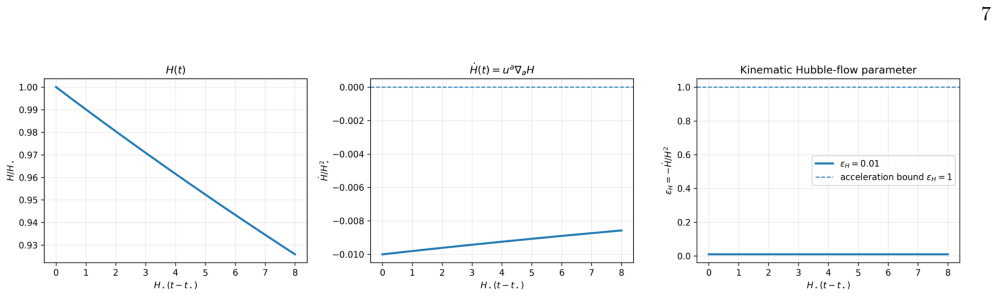
Quasi-de Sitter background H_⋆ and ϵ_H = ϵ_H=10⁻² used in Fig. 3; H_⋆ set by hand
The Hubble evolution H(t)=H⋆/[1+ϵ_H H⋆(t−t⋆)] is assumed in App. D, not derived from the continuation equations.

assumptions (5)

domain assumption The continued metric ĝ_ab = g_ab − Θ u_a u_b satisfies vacuum Einstein equations Ĝ_ab(ĝ)=0 (Eq. 7).
The entire effective source T_ab=Ĝ−G and all subsequent fluid variables depend on this postulate. It is motivated by no-boundary-type thinking but not derived.
domain assumption Θ, K_ab, a_a and their first u-derivatives are bounded and Θ is at least C² near Σ0.
Used in App. A to prove the Kretschmann scalar remains finite at the degenerate hypersurface and hence that Σ0 is curvature-regular.
ad hoc to paper Near-FRW, near-geodesic scaling: ε=1+Θ≪1, σ_K≪1, σ_a≪1, with q^a=O(σ_a) and π^{ab}=O(σ_K+σ_a).
Justifies keeping only the isotropic sector (ρ,P) in the inflationary analysis. The paper shows these corrections are formally subleading but does not prove that a solution of the full continuation lies in this regime.
ad hoc to paper Quasi-de Sitter background during the geometric window: |Ḣ| ≤ ϵ_eff H⋆² on [t⋆,t_end].
Used in App. D to convert Δt_inf into an e-fold estimate N_e ≈ H⋆Δt_inf. The paper states this is a kinematic assumption, not a consequence of the mechanism.
domain assumption Closed, curvature-dominated initial data (compact S³, aH≪1) so that Δ>0.
Needed for ρ≃Δ/(2ε)>0 and for the non-phantom inflationary window; the paper notes that a flat slow-roll background gives Δ≤0 and the mechanism fails.

invented entities (1)

Scalar interpolator Θ(t)
purpose: Smoothly changes the metric signature from Euclidean (Θ→−2) to Lorentzian (Θ→0) across the transition surface at Θ=−1.
Θ is introduced by hand with no dynamics, no Lagrangian, and no observational handle. The choice among tanh, logistic, and arctan profiles is purely ad hoc, and the paper provides no independent evidence for any particular profile.

how reviews work

0 comments

Cite this review

Pith. "Pith review of Inflation from Covariant Signature Change: A Geometric Mechanism." pith.science (2026). https://pith.science/paper/7AS65QNR

@misc{pith2026260701274,
  author       = {Pith},
  title        = {Pith review of: Inflation from Covariant Signature Change: A Geometric Mechanism},
  year         = {2026},
  howpublished = {\url{https://pith.science/paper/7AS65QNR}},
  note         = {Machine review of arXiv:2607.01274}
}

read the original abstract

We present a covariant mechanism in which a smooth change of metric signature, from a Euclidean to a Lorentzian regime, drives a finite interval of accelerated expansion. The transition, encoded by a scalar interpolator along a timelike congruence, occurs on a codimension-one hypersurface where the continued metric is degenerate but curvature invariants remain finite, so the surface is curvature-regular. Using this covariant continuation, we rewrite the Einstein tensor of the continued metric as a localized, interpolator-dependent effective source for the post-transition Lorentzian branch, yielding a purely geometric stress tensor supported near the crossing. In the Lorentzian regime, we derive a model-independent, local criterion for acceleration: inflation persists while the interpolator's slope exceeds a critical value fixed by the extrinsic curvature and the spatial Ricci curvature on the initial hypersurface, and ends when this inequality is first saturated. Standard smooth profiles (tanh, generalized logistic, and power-law/arctan) admit closed-form expressions for the proper-time duration of the accelerated epoch, showing that, for fixed geometric data, the profile shape controls this duration. The construction provides a non-singular, inflaton-free route from a regular Euclidean origin to an early Lorentzian phase of accelerated expansion, in a manner compatible with no--boundary--type boundary conditions.

Figures

Figures reproduced from arXiv: 2607.01274 by the authors.

**Figure 2.** FIG. 2 [PITH_FULL_IMAGE:figures/full_fig_p005_2.png] view at source ↗

**Figure 3.** FIG. 3 [PITH_FULL_IMAGE:figures/full_fig_p007_3.png] view at source ↗

Figures from the paper (1 more)

**Figure 5.** Figure 5: FIG. 5 [PITH_FULL_IMAGE:figures/full_fig_p008_5.png]

Review history (2 revisions) →

Discussion (0). Sign in to comment.

Reference graph

Works this paper leans on

32 extracted references · 15 linked inside Pith

[1]

Lorentzian metric signa- ture is (−,+,+,+) and Euclidean metric signature is (+,+,+,+)

Conventions Except when indicated otherwise, we work in units withc= 1 andℏ= 1. Lorentzian metric signa- ture is (−,+,+,+) and Euclidean metric signature is (+,+,+,+). The projection tensor onto the spatial hy- persurfaces orthogonal to the preferred congruenceu a is hab ≡g ab +u aub,(A1) and our convention for the extrinsic curvature of these hypersurfac...
[2]

degenerate but non–singular

Useful formulae We summarize here the main geometric identities for the class of covariant continued metricsbg ab used in the main text (see also Ref. [11]). The covariant continuation is defined by bgab =g ab −Θu aub,bg ab =g ab +F tatb, t a =g abub, (A3) with F= Θ 1 + Θ, ˙F= ˙Θ (1 + Θ)2 ,(A4) and ∇aF=− ˙F ta,∇ a ˙F=− ¨F ta − ˙F aa.(A5) Hereu a is the (u...
[3]

Geometric decomposition and small parameters We introduce two independent small, dimensionless parameters:σ K (anisotropy of the extrinsic curvature) andσ a (non–geodesicity ofu a). Extrinsic curvature.The extrinsic curvature of the ua–orthogonal slices is decomposed as Kmn = K 3 hmn +σ K ¯Kmn, h mn ¯Kmn = 0,(B2) whereK≡g mnKmn is the expansion scalar of ...
[4]

Heat fluxq m From Sec. III the heat flux is qm = Θa nKmn.(B5) Substituting (B2) and (B4) yields qm = Θ (σa¯an) K 3 hmn +σ K ¯Kmn =σ a Θ K 3 ¯am +σ aσK Θ ¯an ¯Kmn.(B6) Since Θ,K, ¯a m and ¯Kmn are assumed bounded near Σ0, there exists a constantC q >0 such that, in a local orthonormal frame, |qm| ≤Cq σa ⇒q m =O(σ a),(B7) Thus the heat flux is linearly supp...
[5]

III is πmn = Θ " 2t(mKn)a∇uua −KK mn − ∇uKmn + hmn 3 ∇uK+K 2 # + ˙Θ 6 (Kh mn −3K mn),(B8) with∇ u ≡u a∇a

Anisotropic stressπ mn The anisotropic stress tensor derived in Sec. III is πmn = Θ " 2t(mKn)a∇uua −KK mn − ∇uKmn + hmn 3 ∇uK+K 2 # + ˙Θ 6 (Kh mn −3K mn),(B8) with∇ u ≡u a∇a. For an exactly isotropic case, it is straightforward to check thatπ mn = 0 due to non-trivial cancellations among the terms in (B8). We now perturb around this isotropic, geodesic co...
[6]

III, the effective energy density can be writ- ten as ρ= F 2 ∇mam − (3)R+ Θ∇ uK , F≡ Θ 1 + Θ

Comparison with the isotropic energy density From Sec. III, the effective energy density can be writ- ten as ρ= F 2 ∇mam − (3)R+ Θ∇ uK , F≡ Θ 1 + Θ. (B12) Near Σ0 we have Θ =−1 +εand F= −1 +ε ε =− 1 ε + 1.(B13) Usinga m =σ a¯am we obtain ∇mam =O(σ a).(B14) It is convenient to introduce ∆≡ ∇ uK+ (3)R,(B15) Hence ρ= 1 2 − 1 ε + 1 −∆ +∇ mam +ε∇ uK = ∆ 2ε +O ...
[7]

Definition and slope

T anh interpolator a. Definition and slope. Θtanh(t;λ) = tanh(λt)−1, S(t) = ˙Θ(t) =λsech 2(λt), S(0+) =λ. (C1) The microscopic transition width scales as ∆t tr ∼λ −1. 12 b. Inflation window and end time.Inflation requires Sth < S(t)≤S c, i.e. λ >Sc 3 andλ≤S c (to avoidw <−1).(C2) The end time is fixed byS(t end) =S th: sech2 λtend = Sth λ , ∆t(tanh) inf =...
[8]

Generalized logistic interpolator a. Definition and slope.To interpolate from Eu- clidean to Lorentzian across Θ =−1 one may consider ΘGL(t;a, b, m) = 2 1 + exp −a(t/b)m −2, a, b >0, modd integer, (C4) with derivative S(t)≡ ˙Θ(t) = 2am bm t m−1e−a(t/b)m 1 +e −a(t/b)m 2 , S(0+) =    a 2b , m= 1, 0, m≥3 odd. (C5) Form= 1 one has S(t) = a 2b sech2 at 2b ,...

Show all 32 references

[9]

Definition and slope

Power–law (arctan) interpolator a. Definition and slope. ΘPL(t;λ) = 2 π arctan(λt)−1, S(t) = ˙Θ(t) = 2 π λ 1 +λ 2t2 , S(0+) = 2 π λ. (C7) This profile has Θ(0) =−1 and Θ→0 − ast→+∞. b. Inflation window and end time.Inflation occurs only while Sc 3 < 2 π λ≤S c ⇐ ⇒ π 2 Sc 3 < λ≤...
[10]

Geometric scale and quasi–de Sitter regime In a closed FR W background with expansion rateH and curvature (3)R= 6/a 2 one hasK= 3Hand ∆ =∇ uK+ (3)R= 3 ˙H+ 6 a2 .(D2) It is convenient to introduce the geometric deviation pa- rameter ϵG ≡ ∆ 3H 2 = ˙H H 2 + 2 a2H 2 ,∆ = 3ϵ GH 2,(...
[11]

(D1) gives Ne = 1 ϵH ln 1 +ϵ H H⋆∆tinf ,∆t inf ≡t end −t ⋆

Constant-ϵ H toy model As a simple check of the quasi–de Sitter estimate, con- sider a purely kinematic toy model with constant ϵH ≡ − ˙H H 2 = const,(D13) so that ˙H=−ϵ H H 2 and henceH(t) =H ⋆/[1+ϵ H H⋆(t− t⋆)].Substituting into Eq. (D1) gives Ne = 1 ϵH ln 1 +ϵ H H⋆∆tinf ,∆t...
[12]

relative corrections∼ϵ eff Ne

Summary of geometric scaling Collecting the frozen-threshold expression results, the two representative interpolators yield N (tanh) e ≈0.76 ε ϵG , N (PL) e ≈0.60 ε ϵG ,(D17) up to absolute corrections of orderϵ eff H 2 ⋆ ∆t2 inf ∼ϵ eff N 2 e , i.e. relative corrections∼ϵ eff ...
[13]

Remark on moving thresholds The closed-form estimates above treatS th andS c as approximately fixed over the interval during which the interpolator slope is compared with the threshold. This 14 is a useful local analytic expression, but in a curvature- supported closed branch ...
[14]

J. B. Hartle and S. W. Hawking, Physical Review D28, 2960 (1983)

1983
[15]

G. W. Gibbons and J. B. Hartle, Physical Review D42, 2458 (1990)

1990
[16]

Bojowald and G

M. Bojowald and G. M. Paily, Phys. Rev. D86, 104018 (2012), arXiv:1112.1899 [gr-qc]

2012 arXiv
[17]

Zhang, Phys

F. Zhang, Phys. Rev. D100, 064043 (2019), arXiv:1909.10669 [gr-qc]

2019 arXiv
[18]

Ashtekar and J

A. Ashtekar and J. Lewandowski, Classical and Quantum Gravity21, R53 (2004), arXiv:gr-qc/0404018

2004 arXiv
[19]

Cailleteau, J

T. Cailleteau, J. Mielczarek, A. Barrau, and J. Grain, Classical and Quantum Gravity29, 095010 (2012), arXiv:1111.3535 [gr-qc]

2012 arXiv
[20]

Visser, arXiv:1702.05572 [gr-qc]

M. Visser, arXiv:1702.05572 [gr-qc]

arXiv
[21]

Samuel, Class

J. Samuel, Class. Quant. Grav.33, 015006 (2016), arXiv:1510.07365 [gr-qc]

2016 arXiv
[22]

Kothawala, Class

D. Kothawala, Class. Quant. Grav.35, 03LT01 (2018), arXiv:1705.02504 [gr-qc]

2018 arXiv
[23]

Kothawala, Phys

D. Kothawala, Phys. Rev. D97, 124062 (2018), arXiv:1802.07055 [gr-qc]

2018 arXiv
[24]

Singh and D

R. Singh and D. Kothawala, Eur. Phys. J. C83, 194 (2023), arXiv:2010.01822 [gr-qc]

2023 arXiv
[25]

M. Mars, J. M. M. Senovilla, and R. Vera, Phys. Rev. Lett.86, 4219 (2001), arXiv:gr-qc/0012099

2001 arXiv
[26]

M. Mars, J. M. M. Senovilla, and R. Vera, Phys. Rev. D76, 044029 (2007), arXiv:0705.3380 [hep-th]

2007 arXiv
[27]

M. Mars, J. M. M. Senovilla, and R. Vera, Phys. Rev. D77, 027501 (2008), arXiv:0710.0820 [gr-qc]

2008 arXiv
[28]

M. Mars, J. M. M. Senovilla, and R. Vera, EAS Publ. Ser.30, 307 (2008), arXiv:0712.1462 [gr-qc]

2008 arXiv
[29]

S. A. Hayward, Class. Quant. Grav.9, 1851 (1992)

1992
[30]

Bondarenko, Universe8, 497 (2022), arXiv:2111.06095 15 [gr-qc]

S. Bondarenko, Universe8, 497 (2022), arXiv:2111.06095 15 [gr-qc]

2022 arXiv
[31]

Embacher, Physical Review D51, 6764 (1995)

F. Embacher, Physical Review D51, 6764 (1995)

1995
[32]

J. J. Halliwell, J. B. Hartle, and T. Hertog, Phys. Rev. D99, 043526 (2019), arXiv:1812.01760 [hep-th]

2019 arXiv

Pith tools

Reviewed August 2, 2026 · model on record in the stance chip above.

[1] [1]

Lorentzian metric signa- ture is (−,+,+,+) and Euclidean metric signature is (+,+,+,+)

Conventions Except when indicated otherwise, we work in units withc= 1 andℏ= 1. Lorentzian metric signa- ture is (−,+,+,+) and Euclidean metric signature is (+,+,+,+). The projection tensor onto the spatial hy- persurfaces orthogonal to the preferred congruenceu a is hab ≡g ab +u aub,(A1) and our convention for the extrinsic curvature of these hypersurfac...

[2] [2]

degenerate but non–singular

Useful formulae We summarize here the main geometric identities for the class of covariant continued metricsbg ab used in the main text (see also Ref. [11]). The covariant continuation is defined by bgab =g ab −Θu aub,bg ab =g ab +F tatb, t a =g abub, (A3) with F= Θ 1 + Θ, ˙F= ˙Θ (1 + Θ)2 ,(A4) and ∇aF=− ˙F ta,∇ a ˙F=− ¨F ta − ˙F aa.(A5) Hereu a is the (u...

[3] [3]

Geometric decomposition and small parameters We introduce two independent small, dimensionless parameters:σ K (anisotropy of the extrinsic curvature) andσ a (non–geodesicity ofu a). Extrinsic curvature.The extrinsic curvature of the ua–orthogonal slices is decomposed as Kmn = K 3 hmn +σ K ¯Kmn, h mn ¯Kmn = 0,(B2) whereK≡g mnKmn is the expansion scalar of ...

[4] [4]

Heat fluxq m From Sec. III the heat flux is qm = Θa nKmn.(B5) Substituting (B2) and (B4) yields qm = Θ (σa¯an) K 3 hmn +σ K ¯Kmn =σ a Θ K 3 ¯am +σ aσK Θ ¯an ¯Kmn.(B6) Since Θ,K, ¯a m and ¯Kmn are assumed bounded near Σ0, there exists a constantC q >0 such that, in a local orthonormal frame, |qm| ≤Cq σa ⇒q m =O(σ a),(B7) Thus the heat flux is linearly supp...

[5] [5]

III is πmn = Θ " 2t(mKn)a∇uua −KK mn − ∇uKmn + hmn 3 ∇uK+K 2 # + ˙Θ 6 (Kh mn −3K mn),(B8) with∇ u ≡u a∇a

Anisotropic stressπ mn The anisotropic stress tensor derived in Sec. III is πmn = Θ " 2t(mKn)a∇uua −KK mn − ∇uKmn + hmn 3 ∇uK+K 2 # + ˙Θ 6 (Kh mn −3K mn),(B8) with∇ u ≡u a∇a. For an exactly isotropic case, it is straightforward to check thatπ mn = 0 due to non-trivial cancellations among the terms in (B8). We now perturb around this isotropic, geodesic co...

[6] [6]

III, the effective energy density can be writ- ten as ρ= F 2 ∇mam − (3)R+ Θ∇ uK , F≡ Θ 1 + Θ

Comparison with the isotropic energy density From Sec. III, the effective energy density can be writ- ten as ρ= F 2 ∇mam − (3)R+ Θ∇ uK , F≡ Θ 1 + Θ. (B12) Near Σ0 we have Θ =−1 +εand F= −1 +ε ε =− 1 ε + 1.(B13) Usinga m =σ a¯am we obtain ∇mam =O(σ a).(B14) It is convenient to introduce ∆≡ ∇ uK+ (3)R,(B15) Hence ρ= 1 2 − 1 ε + 1 −∆ +∇ mam +ε∇ uK = ∆ 2ε +O ...

[7] [7]

Definition and slope

T anh interpolator a. Definition and slope. Θtanh(t;λ) = tanh(λt)−1, S(t) = ˙Θ(t) =λsech 2(λt), S(0+) =λ. (C1) The microscopic transition width scales as ∆t tr ∼λ −1. 12 b. Inflation window and end time.Inflation requires Sth < S(t)≤S c, i.e. λ >Sc 3 andλ≤S c (to avoidw <−1).(C2) The end time is fixed byS(t end) =S th: sech2 λtend = Sth λ , ∆t(tanh) inf =...

[8] [8]

Generalized logistic interpolator a. Definition and slope.To interpolate from Eu- clidean to Lorentzian across Θ =−1 one may consider ΘGL(t;a, b, m) = 2 1 + exp −a(t/b)m −2, a, b >0, modd integer, (C4) with derivative S(t)≡ ˙Θ(t) = 2am bm t m−1e−a(t/b)m 1 +e −a(t/b)m 2 , S(0+) =    a 2b , m= 1, 0, m≥3 odd. (C5) Form= 1 one has S(t) = a 2b sech2 at 2b ,...