REVIEW 3 major objections 5 minor 82 references
Weak lensing measurements of the APEX-SZ galaxy cluster sample
T0 review · 3 major / 5 minor · reviewed 2026-08-14 · deepseek-v4-flash
Pith's one-line read A per-galaxy colour-based background selection suppresses cosmic-variance scatter in weak-lensing cluster masses by 20–40%.
desk verdict A careful, useful cluster weak lensing mass catalogue; the headline 20–40% scatter-reduction claim is plausible but only partially validated. read the letter →
The pith
A machine-rendered reading of the paper's core claim, the machinery that carries it, and where it could break.
The reading
What carries the argument
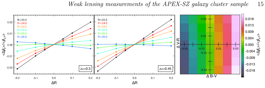
The central object is the per-galaxy angular diameter distance ratio $\beta_g = D_{ds}/D_s$, computed by Eq. (10) as a weighted mean over COSMOS photo-z galaxies inside an elliptical cylinder in colour-colour-magnitude space: $\beta_g = \left(\sum_k w_k \beta(z_d, z_k)\right)/\left(\sum_k w_k\right)$, with a two-dimensional Gaussian weight in the colour plane centred on each source. The cylinder replaces the source-sheet approximation in which one average $\langle\beta\rangle$ is assigned to all galaxies, allowing correlated redshift-distribution changes across a cluster field—cosmic variance, magnification bias, and member contamination—to partly average out. The stellar-locus regression that calibrates the observed colours to the COSMOS photometric system is the enabling step that makes the cylinder match meaningful.
What would settle it
Replace COSMOS with an independent, deeper photo-z reference catalogue (e.g., CFHTLS or a dedicated survey of the same fields) and recompute the $\beta_g$ background selection for the same clusters; if the field-to-field scatter in $\langle\beta\rangle$ is not reduced by 20–40%, or if the mean lensing depth shifts by more than the claimed ~0.5% (about 1.4% in mass), the suppression claim is falsified.
Extended reading notes
Core claim
The paper establishes that a three-band background selection based on an elliptical colour-colour-magnitude cylinder around each galaxy (Eq. 10) estimates $\beta_g$ as a weighted mean over COSMOS photo-z galaxies, recovering the true mean lensing depth $\langle\beta\rangle$ of a cluster field within 0.5% on average. Using nine $30' \times 30'$ COSMOS subfields for clusters at $z = 0.18$, $z = 0.275$, and $z = 0.45$, the cosmic-variance-induced scatter in $\langle\beta\rangle$ between fields is measured to be about 6% for a cluster at $z = 0.45$ with shallow $R \approx 23$ imaging, falling to about 1% at $R = 26$, corresponding to 8.4% and 1.4% scatter in $M_{200}$. The per-galaxy $\beta_g$ selection reduces this scatter by 20–40% relative to using the reference-field mean, and randomized photometry realizations show the remaining scatter is driven by real redshift-distribution variance rather than photometric noise. Combining the selection with a mass-concentration prior from the adopted $c$–$M$ relation yields $M_{200}$ estimates for the 39 APEX-SZ clusters that agree with CCCP and LoCuSS measurements, are lower than Weighing-the-Giants masses, and give concentrations consistent with the adopted $c$–$M$ relation.
Load-bearing premise
The load-bearing premise is that the COSMOS photo-z catalogue, after stellar-locus colour calibration, gives the correct redshift distribution for every region of colour-colour-magnitude space in every observed cluster field; if it does not, every per-galaxy distance ratio $\beta_g$ and hence every cluster mass is biased in the same direction, and the claimed 20–40% scatter reduction would not hold.
Editorial extensions
If this is right
- The 39 masses in Table 2, including the X-ray-selected subsample of 27 clusters, can be used to calibrate SZ and X-ray mass scaling relations at fixed cosmology.
- For deep imaging ($R \approx 26$), cosmic-variance noise in the mean distance ratio drops to about 1%, so per-cluster mass errors become dominated by shape noise rather than redshift-distribution uncertainty.
- Masses derived with and without the mass–concentration prior agree, and recovered concentrations are consistent with the adopted $c$–$M$ relation, supporting the use of such a prior in scaling-relation work.
- The 20–40% scatter reduction is a systematic-floor improvement: applying the same $\beta_g$ selection to larger cluster samples should shrink the cosmic-variance contribution to the mass-scale calibration error.
Reading between the lines
- I infer the method should transfer to other three-band surveys (e.g., wide-field ground-based imaging) as long as a deep, complete photo-z reference catalogue is available; the COSMOS-specific calibration is not essential.
- A testable corollary: using an independent reference catalogue (e.g., CFHTLS or a future deep survey) to compute $\beta_g$ for the same cluster fields should reproduce the 20–40% reduction in field-to-field scatter; if it does not, the suppression is a COSMOS artefact.
- Because all masses scale roughly linearly with $\langle\beta\rangle$, the measured ~0.013 mag colour-calibration scatter translates to ~1.3% changes in $\beta$ and ~2% in mass, so surveys adopting the method should budget colour zero-point calibration as a dominant systematic.
Signed reviews
Editorial analysis
A structured set of objections, weighed in public.
Referee Report
Summary. The paper presents a weak lensing analysis of 39 galaxy clusters from the APEX-SZ survey, using deep three-band optical imaging from WFI and Suprime-Cam. The central methodological novelty is a background-selection scheme in which each source galaxy receives an individual estimate of the angular diameter distance ratio βg, computed by averaging COSMOS photo-z galaxies in a colour-colour-magnitude cylinder around the source (Eq. 10). The authors quantify the variance in the mean lensing depth caused by cosmic variance using nine 30x30 arcmin COSMOS subfields, and report that their selection reduces the field-to-field scatter in ⟨β⟩ by 20-40%, depending on cluster redshift and imaging depth. They derive NFW-based cluster masses with and without a mass-concentration prior, check for residual contamination with shear and density profiles, and compare their masses against LoCuSS, CCCP and WtG. The paper also investigates photometric calibration effects, shear calibration bias, selection-induced bias, and profile-fitting systematics, producing a systematic error budget for the mass scale.
Significance. If the central claim holds, the multi-colour βg estimator suppresses one of the principal systematics in cluster weak lensing mass calibration, and the 39 cluster masses in Table 2 provide a useful anchor for SZ and X-ray scaling relations. The paper's strengths include a careful contamination analysis (individual and stacked shear profiles, galaxy density profiles), consistency checks of recovered concentrations against the Bhattacharya et al. (2013) c-M relation, and comparisons with three independent weak lensing studies showing agreement at the 10-20% level. The paper is also transparent about many systematic uncertainties, presenting a detailed error budget in Sec. 5.7. However, the headline scatter-reduction claim is validated only with a test that uses the COSMOS catalogue both as the reference for the βg estimator and as the 'truth' for the subfields, so the published 20-40% reduction requires stronger independent support before it can be considered established.
major comments (3)
- [Sec. 5.2, Eq. (10)] The central claim that the background selection reduces cosmic-variance scatter by 20-40% is based on a test that is partly circular: the βg estimator in Eq. (10) weights COSMOS photo-z galaxies in a colour-colour cylinder around each source, and the same COSMOS catalogue is then used to define the 'true' mean lensing depth ⟨βtrue⟩i in each of the nine subfields. Because the reference catalogue contains the subfields themselves, any shared large-scale structure or common calibration error will reduce the measured scatter s_meas relative to the cosmic-variance scatter s_cos, biasing the ratio s_meas/s_cos low. The authors acknowledge that the subfields are correlated (Sec. 5.2: 'we expect some correlation between subfields potentially causing an underestimation of the scatter'), but the shared-reference issue is more fundamental and is not quantified. To support the abstract's quantitative claim, the paper should either provide a test where the reference catalogue and the 'truth' are independent, or estimate the magnitude of the circularity bias.
- [Sec. 5.2.1] The CFHTLS deep-field check does not provide an independent measurement of the 20-40% reduction. It measures the scatter in mean β among four 1 deg^2 fields using a simple photo-z cut, and then obtains a '25-30% reduction' by combining a naive √2 area scaling with the assumption that the COSMOS-based reduction applies to CFHTLS. This is an extrapolation, not a direct validation of the βg estimator's performance on independent data. Either the estimator should be run on CFHTLS subfields with an independent reference (e.g., using CFHTLS as both reference and truth in a way that avoids the circularity), or the text should clearly label Sec. 5.2.1 as an order-of-magnitude consistency check rather than a validation.
- [Sec. 5.2, random realization test] The random realization test described in Sec. 5.2 ('we mimic repeated observations of the same subfields... randomly varied the colours of the individual sources in the photo-z catalogues within their photometric errors') addresses photometric noise but not cosmic variance or the shared-reference bias. It shows that the remaining 60-80% scatter is not driven by photometric scatter, but it does not test whether the subfields are representative of independent cluster fields. The conclusion that 'the remaining 60-80% scatter is driven by variance of the redshift distributions' conflates true cosmic variance with the correlated variation captured by the same catalogue. The authors should clarify this distinction or add an external test.
minor comments (5)
- [Abstract and Sec. 1] The abstract contains the typo 'manitude limits' and 'Sunyaev-Zel\textquotesingle dovich'; these should be corrected to 'magnitude' and 'Sunyaev-Zel\'dovich'.
- [Sec. 2.1] There are several typos in this section, including 'Repetititon test' and 'relativie zero points'; these should be fixed.
- [Sec. 5.2] The text uses 'lesning depth' (likely 'lensing depth') and 'string function' (likely 'strong function'); the axes in Fig. 10 are labelled with LaTeX macros such as '/u1D703' and '/u1D737' that are not rendered in the compiled PDF, making the figure difficult to interpret.
- [Sec. 6.1.1] The phrase 'A907 strikes out from the distribution' should probably read 'A907 stands out from the distribution' or 'is an outlier'.
- [Fig. 7 and Fig. 8 captions] The captions for Fig. 7 and Fig. 8 contain garbled text with repeated cluster names and inline math that is not typeset; they need to be rewritten clearly.
Circularity Check
The 20-40% cosmic-variance scatter reduction is validated against the same COSMOS catalogue that defines the estimator; the CFHTLS uncertainty inherits this self-referential reduction, so the headline claim is partly circular.
-
self definitional
[Secs. 4.1-4.2 (Eq. 10) and Sec. 5.2]
"As reference photo-z catalogue we chose the COSMOS photo-z catalogue (Ilbert et al. 2009) ... In order to estimate the level of scatter in ⟨β⟩ that is induced by the cosmic variance and how far our background selection can reduce the scatter, we explored the behaviour of this quantity in 9 individual subfields of the COSMOS field. ... Afterwards, we measure the mean lensing depth ⟨βmeas⟩i based on our method and the mean lensing depth ⟨βtrue⟩i obtained by using directly the COSMOS redshifts of each galaxy for each field i."
The estimator βg in Eq. (10) is a weighted mean over COSMOS photo-z galaxies inside a colour-colour cylinder around each source. The validation in Sec. 5.2 computes ⟨βmeas⟩i by applying this estimator to nine COSMOS subfields and compares it with ⟨βtrue⟩i obtained 'by using directly the COSMOS redshifts of each galaxy for each field i'. Since the subfields are subsets of the same COSMOS catalogue that defines the weighting reference, the 'true' field-to-field scatter and the reference distribution are the same data product. The quoted 20-40% scatter reduction therefore measures partly how the estimator's colour smoothing regresses the reference toward its own mean, not an independent suppression of cosmic variance in external fields.
-
other
[Sec. 5.2.1 and Sec. 5.7]
"As the COSMOS catalogue is about twice the size of a single CFHTLS deep field, the expected impact of cosmic variance is therefore lower. Further, as shown in Fig. 10, our method is able to compensate for 25−30% of the scatter introduced by cosmic variance. Naively imposing a √2 scaling in area and a 25% reduction thanks to our method results in an estimated 1.4% uncertainty caused by cosmic variance within the limited size of the reference catalogue."
The final cosmic-variance uncertainty of 1.4% in β, which is used to derive the 2% mass uncertainty in Sec. 5.7, is not obtained from the external CFHTLS fields alone. It combines the CFHTLS field-to-field scatter with 'a 25% reduction thanks to our method' taken from Fig. 10, i.e., from the self-referential COSMOS subfield test. The external data therefore only calibrate the raw scatter; the claimed reduction factor, which is the load-bearing part of the uncertainty estimate, is inherited from the circular Sec. 5.2 comparison. This makes the propagated uncertainty partially circular as well.
full rationale
The paper's cluster mass measurements are benchmarked against independent external samples (CCCP, LoCuSS, WtG) and the shear pipeline, PSF correction, and mass-concentration prior come from external or previously established work, so the mass catalogue itself is not circular. The circularity is concentrated in the novel methodological claim: the '20-40% reduction' of cosmic-variance-induced scatter in the mean lensing depth. That claim is tested by applying the colour-cylinder estimator, defined from the COSMOS photo-z catalogue, to nine COSMOS subfields and comparing against 'true' mean lensing depths taken from the same COSMOS redshifts. The reference and the truth are the same data product, so the measured reduction is partly a self-consistency or smoothing effect rather than an external validation. The CFHTLS check is genuinely independent for the raw field-to-field scatter, but the final uncertainty estimate imports the 25-30% reduction factor from the self-referential COSMOS test, so the external data do not independently rescue the headline reduction. This is a partial circularity of the central scatter-reduction claim, but it does not invalidate the mass measurements, which rest on independent comparisons and established external priors. Score 5 reflects one load-bearing validation loop in an otherwise externally anchored analysis.
Assumptions & free parameters
free parameters (5)
- Global shear calibration factor f0 =
1.08 (adopted from Israel et al. 2010)
- Per-cluster beta_cut and p_cut =
Values in Table 2; beta_cut ranges from 0.15 to 0.69, p_cut from 0.2 to 0.8
- Shape catalogue S/N threshold =
5.5 for the conservative model, 4.5 for the S/N-optimized model
- Selection offset delta_z in beta_cut =
0.04 for conservative model, 0.0 for optimized model
- Mass-concentration prior parameters =
c200(nu)=5.9 nu^-0.41 D(z)^0.54 with scatter 0.33c (Bhattacharya et al. 2013)
assumptions (5)
- domain assumption The COSMOS photo-z catalogue (Ilbert et al. 2009), after stellar locus calibration, represents the true joint distribution of colour, magnitude and redshift for galaxies in each observed cluster field.
- domain assumption Galaxy clusters are adequately described by an NFW density profile over the fitted radial range.
- domain assumption The Bhattacharya et al. (2013) mass-concentration relation provides a suitable prior for the sample.
- domain assumption The KSB+ shape measurement pipeline, with the adopted f0=1.08 calibration and a S/N threshold, returns unbiased shear estimates.
- domain assumption A flat LambdaCDM cosmology with Omega_m=0.3, Omega_Lambda=0.7, h=0.7 is assumed.
Cite this review
Pith. "Pith review of Weak lensing measurements of the APEX-SZ galaxy cluster sample." pith.science (2026). https://pith.science/paper/A4MJ7ZPX
@misc{pith2026190810114,
  author       = {Pith},
  title        = {Pith review of: Weak lensing measurements of the APEX-SZ galaxy cluster sample},
  year         = {2026},
  howpublished = {\url{https://pith.science/paper/A4MJ7ZPX}},
  note         = {Machine review of arXiv:1908.10114}
}
abstract
We present a weak lensing analysis for galaxy clusters from the APEX-SZ survey. For $39$ massive galaxy clusters that were observed via the Sunyaev-Zel\textquotesingle dovich effect (SZE) with the APEX telescope, we analyse deep optical imaging data from WFI(@2.2mMPG/ESO) and Suprime-Cam(@SUBARU) in three bands. The masses obtained in this study, including an X-ray selected subsample of 27 clusters, are optimised for and used in studies constraining the mass to observable scaling relations at fixed cosmology. A novel focus of our weak lensing analysis is the multi-colour background selection to suppress effects of cosmic variance on the redshift distribution of source galaxies. We investigate the effects of cluster member contamination through galaxy density, shear profile, and recovered concentrations. We quantify the impact of variance in source redshift distribution on the mass estimate by studying nine sub-fields of the COSMOS survey for different cluster redshift and manitude limits. We measure a standard deviation of $\sim 6$\% on the mean angular diameter distance ratio for a cluster at $z\!=\!0.45$ and shallow imaging data of $R\!\approx\!23$ mag. It falls to $\sim 1$\% for deep, $R=26$ mag, observations. This corresponds to 8.4\% and 1.4\% scatter in $M_{200}$. Our background selection reduces this scatter by $20-40$\%, depending on cluster redshift and imaging depth. We derived cluster masses with and without using a mass concentration relation and find consistent results, and concentrations consistent with the used mass-concentration relation.
Figures


Figures from the paper (12 more)




Reference graph
Works this paper leans on
-
[1]
write newline
" write newline "" before.all 'output.state := FUNCTION fin.entry write newline FUNCTION new.block output.state before.all = 'skip after.block 'output.state := if FUNCTION new.sentence output.state after.block = 'skip output.state before.all = 'skip after.sentence 'output.state := if if FUNCTION not #0 #1 if FUNCTION and 'skip pop #0 if FUNCTION or pop #1...
-
[2]
write newline
" write newline "" before.all 'output.state := FUNCTION fin.entry write newline FUNCTION new.block output.state before.all = 'skip after.block 'output.state := if FUNCTION new.sentence output.state after.block = 'skip output.state before.all = 'skip after.sentence 'output.state := if if FUNCTION not #0 #1 if FUNCTION and 'skip pop #0 if FUNCTION or pop #1...
-
[3]
Albrecht A., et al., 2006, ArXiv astro-ph/0609591, http://adsabs.harvard.edu/abs/2006astro.ph..9591A
arXiv 2006
-
[4]
Applegate D. E., et al., 2014, @doi [ ] 10.1093/mnras/stt2129 , http://adsabs.harvard.edu/abs/2014MNRAS.439...48A 439, 48
-
[5]
Baade D., et al., 1999, The Messenger, http://esoads.eso.org/abs/1999Msngr..95...15B 95, 15
work page 1999
-
[6]
Bah \'e Y. M., McCarthy I. G., King L. J., 2012, @doi [ ] 10.1111/j.1365-2966.2011.20364.x , http://adsabs.harvard.edu/abs/2012MNRAS.421.1073B 421, 1073
-
[7]
P., 2005, @doi [ ] 10.1051/0004-6361:20041643 , http://cdsads.u-strasbg.fr/abs/2005A
Bardeau S., Kneib J.-P., Czoske O., Soucail G., Smail I., Ebeling H., Smith G. P., 2005, @doi [ ] 10.1051/0004-6361:20041643 , http://cdsads.u-strasbg.fr/abs/2005A
-
[8]
Bartelmann M., 1996, , http://cdsads.u-strasbg.fr/abs/1996A
work page 1996
Show all 82 references
-
[9]
Bartelmann M., Schneider P., 2001, @doi [ ] 10.1016/S0370-1573(00)00082-X , http://adsabs.harvard.edu/abs/2001PhR...340..291B 340, 291
2001 doi
-
[10]
R., Kravtsov A
Becker M. R., Kravtsov A. V., 2011, @doi [ ] 10.1088/0004-637X/740/1/25 , http://adsabs.harvard.edu/abs/2011ApJ...740...25B 740, 25
2011 doi
-
[11]
N., et al., 2016, @doi [ ] 10.1093/mnras/stw1158 , http://adsabs.harvard.edu/abs/2016MNRAS.460.3432B 460, 3432
Bender A. N., et al., 2016, @doi [ ] 10.1093/mnras/stw1158 , http://adsabs.harvard.edu/abs/2016MNRAS.460.3432B 460, 3432
2016 doi
-
[12]
A., et al., 2014, in Millimeter, Submillimeter, and Far-Infrared Detectors and Instrumentation for Astronomy VII
Benson B. A., et al., 2014, in Millimeter, Submillimeter, and Far-Infrared Detectors and Instrumentation for Astronomy VII. p. 91531P ( @eprint arXiv 1407.2973 ), @doi 10.1117/12.2057305
2014 arXiv
-
[13]
Bhattacharya S., Habib S., Heitmann K., Vikhlinin A., 2013, @doi [ ] 10.1088/0004-637X/766/1/32 , http://adsabs.harvard.edu/abs/2013ApJ...766...32B 766, 32
2013 doi
-
[14]
Bocquet S., et al., 2018, arXiv e-prints, http://adsabs.harvard.edu/abs/2018arXiv181201679B
2018
-
[15]
Cavaliere A., Fusco-Femiano R., 1978, , http://cdsads.u-strasbg.fr/abs/1978A
1978
-
[16]
Clowe D., Schneider P., 2001, @doi [ ] 10.1051/0004-6361:20011310 , http://adsabs.harvard.edu/abs/2001A
2001 doi
-
[17]
Clowe D., Schneider P., 2002, @doi [ ] 10.1051/0004-6361:20021137 , http://adsabs.harvard.edu/abs/2002A
2002 doi
-
[18]
Costanzi M., et al., 2018, arXiv e-prints, http://adsabs.harvard.edu/abs/2018arXiv181009456C
2018
-
[19]
Coupon J., et al., 2009, @doi [ ] 10.1051/0004-6361/200811413 , http://adsabs.harvard.edu/abs/2009A
2009 doi
-
[20]
M., et al
Cutri R. M., et al. 2014, VizieR Online Data Catalog, http://adsabs.harvard.edu/abs/2014yCat.2328....0C 2328
2014
-
[21]
Dark Energy Survey Collaboration et al., 2016, @doi [ ] 10.1093/mnras/stw641 , http://adsabs.harvard.edu/abs/2016MNRAS.460.1270D 460, 1270
2016 doi
-
[22]
P., et al., 2019, @doi [ ] 10.1093/mnras/sty3088 , http://adsabs.harvard.edu/abs/2019MNRAS.483.2871D 483, 2871
Dietrich J. P., et al., 2019, @doi [ ] 10.1093/mnras/sty3088 , http://adsabs.harvard.edu/abs/2019MNRAS.483.2871D 483, 2871
2019 doi
-
[23]
Dobbs M., et al., 2006, @doi [ ] 10.1016/j.newar.2006.09.029 , http://adsabs.harvard.edu/abs/2006NewAR..50..960D 50, 960
2006 doi
-
[24]
A., et al., 2012, @doi [Review of Scientific Instruments] 10.1063/1.4737629 , http://adsabs.harvard.edu/abs/2012RScI...83g3113D 83, 073113
Dobbs M. A., et al., 2012, @doi [Review of Scientific Instruments] 10.1063/1.4737629 , http://adsabs.harvard.edu/abs/2012RScI...83g3113D 83, 073113
2012 doi
-
[25]
Erben T., van Waerbeke L., Bertin E., Mellier Y., Schneider P., 2001, @doi [ ] 10.1051/0004-6361:20010013 , http://cdsads.u-strasbg.fr/abs/2001A
2001 doi
-
[26]
Erben T., et al., 2005, @doi [Astronomische Nachrichten] 10.1002/asna.200510396 , http://adsabs.harvard.edu/abs/2005AN....326..432E 326, 432
2005 doi
-
[27]
Ettori S., Gastaldello F., Leccardi A., Molendi S., Rossetti M., Buote D., Meneghetti M., 2010, @doi [ ] 10.1051/0004-6361/201015271 , http://adsabs.harvard.edu/abs/2010A
2010 doi
-
[28]
Gitti M., Piffaretti R., Schindler S., 2007, @doi [ ] 10.1051/0004-6361:20077580 , http://adsabs.harvard.edu/abs/2007A
2007 doi
-
[29]
Gruen D., et al., 2014, @doi [ ] 10.1093/mnras/stu949 , http://adsabs.harvard.edu/abs/2014MNRAS.442.1507G 442, 1507
2014 doi
-
[30]
, Schilke P., Menten K., Cesarsky C., Booth R., 2006, @doi [ ] 10.1051/0004-6361:20065420 , http://adsabs.harvard.edu/abs/2006A
G \"u sten R., Nyman L. ., Schilke P., Menten K., Cesarsky C., Booth R., 2006, @doi [ ] 10.1051/0004-6361:20065420 , http://adsabs.harvard.edu/abs/2006A
2006 doi
-
[31]
Hartlap J., Schrabback T., Simon P., Schneider P., 2009, @doi [ ] 10.1051/0004-6361/200911697 , http://adsabs.harvard.edu/abs/2009A
2009 doi
-
[32]
J., 2004, in Hilditch R
Henry T. J., 2004, in Hilditch R. W., Hensberge H., Pavlovski K., eds, Astronomical Society of the Pacific Conference Series Vol. 318, Spectroscopically and Spatially Resolving the Components of the Close Binary Stars. pp 159--165
2004
-
[33]
Heymans C., et al., 2006, @doi [ ] 10.1111/j.1365-2966.2006.10198.x , http://cdsads.u-strasbg.fr/abs/2006MNRAS.368.1323H 368, 1323
2006
-
[34]
W., Stubbs C
High F. W., Stubbs C. W., Rest A., Stalder B., Challis P., 2009, @doi [ ] 10.1088/0004-6256/138/1/110 , http://adsabs.harvard.edu/abs/2009AJ....138..110H 138, 110
2009 doi
-
[35]
Hoekstra H., Mahdavi A., Babul A., Bildfell C., 2012, @doi [ ] 10.1111/j.1365-2966.2012.22072.x , http://adsabs.harvard.edu/abs/2012MNRAS.427.1298H 427, 1298
2012
-
[36]
Hoekstra H., Herbonnet R., Muzzin A., Babul A., Mahdavi A., Viola M., Cacciato M., 2015, @doi [ ] 10.1093/mnras/stv275 , http://adsabs.harvard.edu/abs/2015MNRAS.449..685H 449, 685
2015 doi
-
[37]
Ilbert O., et al., 2006, @doi [ ] 10.1051/0004-6361:20065138 , http://cdsads.u-strasbg.fr/abs/2006A
2006 doi
-
[38]
Ilbert O., et al., 2009, @doi [ ] 10.1088/0004-637X/690/2/1236 , http://cdsads.u-strasbg.fr/abs/2009ApJ...690.1236I 690, 1236
2009 doi
-
[39]
Israel H., et al., 2010, @doi [ ] 10.1051/0004-6361/200913667 , http://adsabs.harvard.edu/abs/2010A
2010 doi
-
[40]
H., Vikhlinin A., Sarazin C
Israel H., Erben T., Reiprich T. H., Vikhlinin A., Sarazin C. L., Schneider P., 2012, @doi [ ] 10.1051/0004-6361/201118676 , http://adsabs.harvard.edu/abs/2012A
2012 doi
-
[41]
Juri \'c M., et al., 2008, @doi [ ] 10.1086/523619 , http://adsabs.harvard.edu/abs/2008ApJ...673..864J 673, 864
2008 doi
-
[42]
Kaiser N., Squires G., Broadhurst T., 1995, @doi [ ] 10.1086/176071 , http://adsabs.harvard.edu/abs/1995ApJ...449..460K 449, 460
1995 doi
-
[43]
Komatsu E., et al., 2011, @doi [ ] 10.1088/0067-0049/192/2/18 , http://adsabs.harvard.edu/abs/2011ApJS..192...18K 192, 18
2011 doi
-
[44]
E., Le Brun A
Lee B. E., Le Brun A. M. C., Haq M. E., Deering N. J., King L. J., Applegate D., McCarthy I. G., 2018, @doi [ ] 10.1093/mnras/sty1377 , http://adsabs.harvard.edu/abs/2018MNRAS.tmp.1333L
2018 doi
-
[46]
Medezinski E., Broadhurst T., Umetsu K., Oguri M., Rephaeli Y., Ben \' tez N., 2010, @doi [ ] 10.1111/j.1365-2966.2010.16491.x , http://adsabs.harvard.edu/abs/2010MNRAS.405..257M 405, 257
2010
-
[47]
Medezinski E., et al., 2018, @doi [ ] 10.1093/pasj/psy009 , http://adsabs.harvard.edu/abs/2018PASJ..tmp...23M
2018 doi
-
[48]
Melchior P., et al., 2017, @doi [ ] 10.1093/mnras/stx1053 , http://adsabs.harvard.edu/abs/2017MNRAS.469.4899M 469, 4899
2017 doi
-
[49]
Miyazaki S., et al., 2002, , http://adsabs.harvard.edu/abs/2002PASJ...54..833M 54, 833
2002
-
[50]
Nagarajan A., et al., 2018, @doi [ ] 10.1093/mnras/sty1904 , http://adsabs.harvard.edu/abs/2018MNRAS.tmp.1811N
2018 doi
-
[51]
F., Frenk C
Navarro J. F., Frenk C. S., White S. D. M., 1995, , http://cdsads.u-strasbg.fr/abs/1995MNRAS.275..720N 275, 720
1995
-
[52]
F., Frenk C
Navarro J. F., Frenk C. S., White S. D. M., 1996, @doi [ ] 10.1086/177173 , http://cdsads.u-strasbg.fr/abs/1996ApJ...462..563N 462, 563
1996 doi
-
[53]
F., Frenk C
Navarro J. F., Frenk C. S., White S. D. M., 1997, @doi [ ] 10.1086/304888 , http://cdsads.u-strasbg.fr/abs/1997ApJ...490..493N 490, 493
1997 doi
-
[54]
Nulsen P. E. J., Powell S. L., Vikhlinin A., 2010, @doi [ ] 10.1088/0004-637X/722/1/55 , http://adsabs.harvard.edu/abs/2010ApJ...722...55N 722, 55
2010 doi
-
[55]
P., 2016, @doi [ ] 10.1093/mnras/stw1539 , http://adsabs.harvard.edu/abs/2016MNRAS.461.3794O 461, 3794
Okabe N., Smith G. P., 2016, @doi [ ] 10.1093/mnras/stw1539 , http://adsabs.harvard.edu/abs/2016MNRAS.461.3794O 461, 3794
2016 doi
-
[56]
Pacaud F., et al., 2018, @doi [ ] 10.1051/0004-6361/201834022 , http://adsabs.harvard.edu/abs/2018A
2018 doi
-
[57]
Pillepich A., Porciani C., Hahn O., 2010, @doi [ ] 10.1111/j.1365-2966.2009.15914.x , http://cdsads.u-strasbg.fr/abs/2010MNRAS.402..191P 402, 191
2010
-
[58]
Planck Collaboration et al., 2011, @doi [ ] 10.1051/0004-6361/201116458 , http://adsabs.harvard.edu/abs/2011A
2011 doi
-
[59]
Postman M., et al., 2012, @doi [ ] 10.1088/0067-0049/199/2/25 , http://adsabs.harvard.edu/abs/2012ApJS..199...25P 199, 25
2012 doi
-
[60]
L., et al., 2019, @doi [ ] 10.1093/mnras/stz817 , http://adsabs.harvard.edu/abs/2019MNRAS.486...77R 486, 77
Rehmann R. L., et al., 2019, @doi [ ] 10.1093/mnras/stz817 , http://adsabs.harvard.edu/abs/2019MNRAS.486...77R 486, 77
2019 doi
-
[61]
Robertson A., Massey R., Eke V., 2017, @doi [ ] 10.1093/mnras/stw2670 , http://adsabs.harvard.edu/abs/2017MNRAS.465..569R 465, 569
2017 doi
-
[62]
Rosati P., Borgani S., Norman C., 2002, @doi [ ] 10.1146/annurev.astro.40.120401.150547 , http://cdsads.u-strasbg.fr/abs/2002ARA
2002
-
[63]
Schirmer M., 2013, @doi [ ] 10.1088/0067-0049/209/2/21 , http://adsabs.harvard.edu/abs/2013ApJS..209...21S 209, 21
2013 doi
-
[64]
Schirmer M., Erben T., Hetterscheidt M., Schneider P., 2007, @doi [ ] 10.1051/0004-6361:20065955 , http://cdsads.u-strasbg.fr/abs/2007A
2007 doi
-
[65]
Schirmer M., Suyu S., Schrabback T., Hildebrandt H., Erben T., Halkola A., 2010, @doi [ ] 10.1051/0004-6361/200913810 , http://adsabs.harvard.edu/abs/2010A
2010 doi
-
[66]
Springer Berlin Heidelberg, Berlin, Heidelberg, pp 269--451, @doi 10.1007/978-3-540-30310-7_3 , https://doi.org/10.1007/978-3-540-30310-7_3
Schneider P., 2006, Weak Gravitational Lensing. Springer Berlin Heidelberg, Berlin, Heidelberg, pp 269--451, @doi 10.1007/978-3-540-30310-7_3 , https://doi.org/10.1007/978-3-540-30310-7_3
2006 doi
-
[67]
Schneider P., King L., Erben T., 2000, , http://cdsads.u-strasbg.fr/abs/2000A
2000
-
[68]
Schrabback T., et al., 2007, @doi [ ] 10.1051/0004-6361:20065898 , http://cdsads.u-strasbg.fr/abs/2007A
2007 doi
-
[69]
18, Reviews in Modern Astronomy
Schuecker P., 2005, in R \"o ser S., ed., Reviews in Modern Astronomy Vol. 18, Reviews in Modern Astronomy. pp 76--105, @doi 10.1002/3527608966.ch4
2005 doi
-
[70]
Schwan D., et al., 2011, @doi [Review of Scientific Instruments] 10.1063/1.3637460 , http://adsabs.harvard.edu/abs/2011RScI...82i1301S 82, 091301
2011 doi
-
[71]
Schwan D., et al., 2012, The Messenger, http://adsabs.harvard.edu/abs/2012Msngr.147....7S 147, 7
2012
-
[72]
Seitz S., Schneider P., 1996, , http://cdsads.u-strasbg.fr/abs/1996A
1996
-
[73]
Seitz S., Schneider P., 2001, @doi [ ] 10.1051/0004-6361:20010493 , http://cdsads.u-strasbg.fr/abs/2001A
2001 doi
-
[74]
B., 2000, @doi [ ] 10.1086/316595 , http://adsabs.harvard.edu/abs/2000PASP..112..925S 112, 925
Stetson P. B., 2000, @doi [ ] 10.1086/316595 , http://adsabs.harvard.edu/abs/2000PASP..112..925S 112, 925
2000 doi
-
[75]
Umetsu K., Broadhurst T., Zitrin A., Medezinski E., Hsu L.-Y., 2011, @doi [ ] 10.1088/0004-637X/729/2/127 , http://adsabs.harvard.edu/abs/2011ApJ...729..127U 729, 127
2011 doi
-
[76]
M., 2005, @doi [Reviews of Modern Physics] 10.1103/RevModPhys.77.207 , http://adsabs.harvard.edu/abs/2005RvMP...77..207V 77, 207
Voit G. M., 2005, @doi [Reviews of Modern Physics] 10.1103/RevModPhys.77.207 , http://adsabs.harvard.edu/abs/2005RvMP...77..207V 77, 207
2005 doi
-
[77]
O., Brainerd T
Wright C. O., Brainerd T. G., 2000, @doi [ ] 10.1086/308744 , http://cdsads.u-strasbg.fr/abs/2000ApJ...534...34W 534, 34
2000 doi
-
[78]
L., et al., 2010, @doi [ ] 10.1088/0004-6256/140/6/1868 , http://adsabs.harvard.edu/abs/2010AJ....140.1868W 140, 1868
Wright E. L., et al., 2010, @doi [ ] 10.1088/0004-6256/140/6/1868 , http://adsabs.harvard.edu/abs/2010AJ....140.1868W 140, 1868
2010 doi
-
[79]
P., Kneissl R., Okabe N., Dahle H., 2008, @doi [ ] 10.1051/0004-6361:20079103 , http://cdsads.u-strasbg.fr/abs/2008A
Zhang Y.-Y., Finoguenov A., B \"o hringer H., Kneib J.-P., Smith G. P., Kneissl R., Okabe N., Dahle H., 2008, @doi [ ] 10.1051/0004-6361:20079103 , http://cdsads.u-strasbg.fr/abs/2008A
2008 doi
-
[80]
P., Okabe N., Haines C
Ziparo F., Smith G. P., Okabe N., Haines C. P., Pereira M. J., Egami E., 2016, @doi [ ] 10.1093/mnras/stw2192 , http://adsabs.harvard.edu/abs/2016MNRAS.463.4004Z 463, 4004
2016 doi
-
[81]
de Haan T., et al., 2016, @doi [ ] 10.3847/0004-637X/832/1/95 , http://adsabs.harvard.edu/abs/2016ApJ...832...95D 832, 95
2016 doi
-
[82]
van Waerbeke L., White M., Hoekstra H., Heymans C., 2006, @doi [Astroparticle Physics] 10.1016/j.astropartphys.2006.05.008 , http://adsabs.harvard.edu/abs/2006APh....26...91V 26, 91
2006 doi
-
[83]
von der Linden A., et al., 2014, @doi [ ] 10.1093/mnras/stt1945 , http://adsabs.harvard.edu/abs/2014MNRAS.439....2V 439, 2
2014 doi
Reviewed August 14, 2026 · model on record in the stance chip above.
Discussion (0). Continue with ORCID to comment.