REVIEW 2 major objections 5 minor 1 cited by
Multi-Source Urban Traffic Flow Forecasting with Drone and Loop Detector Data
T0 review · 2 major / 5 minor · reviewed 2026-08-10 · deepseek-v4-flash
Pith's one-line read Fusing drone and loop-detector data improves urban traffic forecasts when sensors are sparse and noisy.
desk verdict A useful simulated multi-source traffic benchmark with an honest simple baseline, but the paper's central fusion-advantage claim rests on a 0.01 m/s gap that needs repeated-seed evidence. read the letter →
The pith
A machine-rendered reading of the paper's core claim, the machinery that carries it, and where it could break.
The reading
What carries the argument
The engine of the argument is HiMSNet's two-layer design, built from an LSTM recurrent temporal encoder and graph-convolution message-passing layers. Each sensor modality is encoded separately—loop detectors at 3-minute resolution, drones at 5-second resolution with 1D convolutions to downsample—producing a per-location joint feature; the global layer then exchanges these features across the road graph so each segment's prediction uses its neighbors' states. A regional branch averages the segment features in each of four spatial clusters to forecast region-average speed. The complementary part of the machinery is the dataset pipeline: trajectory splits are summed via Edie's definitions to compute segment speed from drone observations and point speed from loop detectors, so the two modalities measure genuinely different quantities—a whole-segment average versus a single-point sample—which is precisely the gap HiMSNet must bridge.
What would settle it
Re-run the same HiMSNet and training setup on a real urban network with drones and loop detectors at roughly 10% coverage, measuring actual drone segment-speed error and repositioning times, and check whether the fused model beats both single-modality models by the margins reported in Table III. If real drone noise is larger than the simulated 15 percent, or drones take minutes to move between cells, and the multi-source advantage disappears, the central claim is refuted.
Extended reading notes
Core claim
The paper's central claim is that multi-source forecasting—combining loop detector point speeds with drone-measured segment speeds—is better than single-modality forecasting exactly in the regime that matters for deployment: low sensor coverage and noisy measurements. In the clean, full-coverage setting, drone-only inputs are already so good that adding loop detectors brings no segment-level gain (1.00 vs 1.01 MAE at 15 minutes), while loop-only inputs fall behind (1.13). But once coverage drops to 10% and both inputs carry simulated noise, the fused HiMSNet achieves the lowest errors on both tasks and both horizons, and the gap between fused and loop-only widens (1.06 vs 1.12 segment, 0.32 vs 0.41 regional at 15 minutes). A further ablation in which drones are absent from both training and testing—simulating taxi or ride-hailing labels instead—raises regional MAE to 0.56, which the authors read as evidence that drone-quality training labels are necessary to learn the point-to-segment speed translation that loop detectors alone cannot provide.
Load-bearing premise
The paper's conclusion rests on the assumption that real drones can see full road-segment speeds in 220-by-220-meter cells, move between cells every three minutes with no delay, and suffer at most the mild simulated noise, and that the simulated Barcelona network faithfully represents real traffic; that second assumption is asserted, not quantitatively demonstrated.
Editorial extensions
If this is right
- If the claim holds, cities should treat aerial data as a primary traffic-sensing layer, not a luxury: in the simulated 10%-coverage/noisy setting, drone-only forecasts nearly match the fused model on segment-level MAE (1.07 vs 1.06 m/s).
- Adding fixed loop detectors to drone coverage is still worthwhile when coverage is incomplete and noisy, but the extra gain is small—a few hundredths of m/s—so its practical value depends on whether the fixed sensors already exist.
- Segment-level prediction is the hard problem; regional averages are much easier and can hide sensor deficiencies (regional MAE 0.32 vs segment MAE 1.06 under partial/noisy conditions), so evaluations that report only network-level speeds may overstate model quality.
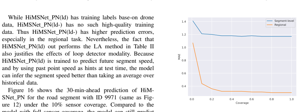
- Sensor coverage has a natural operating point: roughly 20% coverage reproduces full-coverage performance, while 1% coverage collapses toward a constant-prediction baseline, making the 10–20% range the relevant design space.
- A loop-only model trained on drone-derived labels outperforms one trained without such labels, meaning historical drone observations can create high-quality training targets for sensor networks that later run without drones, for example in bad weather.
Reading between the lines
- The paper does not test it, but the 20%-coverage-matches-full-coverage result implies a deployment rule: roughly one aerial monitoring cell per five could suffice for forecasting, with fixed detectors reserved for spots drones cannot see.
- The simulated drone model is optimistic—instant relocation, full-segment visibility, mild noise—so a field trial measuring actual drone repositioning time and per-segment speed error would show whether the reported margins survive in practice.
- The trajectory-split pipeline could be lifted onto real drone trajectory datasets without modification; if it transfers, segment-level forecasting benchmarks could replace point-sensor benchmarks for urban networks.
- The red-light queuing explanation for why loop detectors overestimate segment speed depends on detector placement at segment midpoints; real-world placements vary, so the size of the drone advantage should be re-measured where detectors sit near stop lines.
Editorial analysis
A structured set of objections, weighed in public.
Referee Report
Summary. The paper proposes HiMSNet, a hierarchical graph-based model that fuses simulated drone-derived segment speeds with loop-detector point speeds to predict both segment-level and regional average speeds in a Barcelona Aimsun simulation, which the authors release as the SimBarca dataset. The authors describe the multi-source forecasting formulation, the model architecture, the trajectory-based dataset construction, and a partial-and-noisy (PN) sensing scenario with 10% sensor coverage and multiplicative Gaussian noise. The central claim is that, under partial and noisy sensing, using both drone and loop detector data improves prediction accuracy over either single-modality input, with drone data being the more informative modality.
Significance. If substantiated, the paper would provide a useful benchmark and a simple baseline for multi-source urban traffic forecasting with aerial and ground sensors. The strengths are the detailed trajectory-based dataset construction, the joint treatment of segment-level and regional prediction tasks, a transparent and reproducible architecture, ablation studies, and a coverage sensitivity analysis. The authors state that data and code will be shared, although no link is currently provided. The main limitation is that the central empirical claim currently rests on extremely small metric differences without any uncertainty quantification, so the practical significance of the fusion benefit is not yet established.
major comments (2)
- [Section IV-G, Table III] The evidence for the abstract's improvement claim is the comparison between HiMSNet PN (both modalities) and HiMSNet PN(drone) in Table III: segment 15-min MAE 1.06 vs. 1.07, segment 30-min MAE 1.21 vs. 1.22, regional 15-min MAE 0.32 vs. 0.32, and regional 30-min MAE 0.44 vs. 0.44. These differences are smaller than the differences that motivate the paper, and they are within ordinary run-to-run variation given randomized training, stochastic demand augmentation, random loop detector placement, and multiplicative sensor noise. No standard deviations, repeated-seed results, or significance tests are reported anywhere in the paper. Moreover, in the full-information setting (Table II), the single-modality drone model slightly outperforms the multi-modality model, so the sign of the fusion benefit is not stable across settings. The central claim requires multi-seed results with confidence intervals or a paired significance test; as it stands, the improvement claim is unsupported.
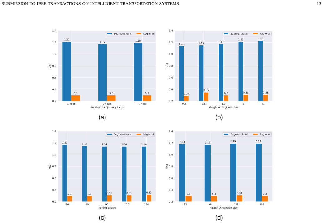
- [Sections III-C3 and IV-F] The PN scenario, which is the only setting where the multi-modality advantage is claimed, is defined by a stylized sensor model: drones observe complete segment speeds in 220x220 m grid cells, receive multiplicative Gaussian noise with standard deviation 0.15, and relocate every 3 minutes with zero travel time, while loop detectors are installed on 10% of segments. The Aimsun model is described as well-calibrated, but no quantitative calibration evidence is provided, and no sensitivity analysis is given for the noise level, grid-cell size, relocation time, or detector placement. Since the central claim is specifically about the PN setting, the claim is only as strong as these assumptions; a sensitivity analysis or validation against real drone and loop detector data is needed to establish that the qualitative conclusion is robust.
minor comments (5)
- [Section II-A] There is a typo in the first paragraph: "within a dinstance" should read "within a distance."
- [Section III-B, Eq. (8)] The normalization factor in Equation (8) is not rendered clearly; the expression "1p D(i) · D(j)" should use an explicit square-root notation, such as 1/sqrt(D(i)D(j)).
- [Section III-B] The sentence stating that missing values are replaced with "learnable neural network parameters of equal size" should clarify whether this is a single learnable embedding per modality or a per-segment parameter, as this affects both the parameter count and the interpretation.
- [Section IV-F] The description of the PN setting does not state how the random sensor placement and multiplicative noise are generated across runs; specifying the random seed policy and whether noise is resampled per sample would improve reproducibility.
- [Section I] The statement that the data, model, and evaluations are openly shared is not verifiable in the current manuscript because no repository link is provided; please provide a link or clearly state that it will be available in a companion repository.
Circularity Check
No significant circularity: predictions are evaluated on held-out simulated runs with independently computed trajectory-based labels.
full rationale
The paper is an empirical evaluation rather than a first-principles derivation. Segment-speed and regional-speed labels are computed from simulated vehicle trajectories via Edie's formula (Eq. 9), independently of the model outputs and test-time inputs. Training and test sets come from disjoint simulation sessions (75 of 101 runs for training), and in the partial/noisy setting the test labels are clean while only the inputs are corrupted, so no test-label information enters training. The Label Average baseline uses the test-set label average, but the paper explicitly calls it the best constant oracle rather than a learned prediction, so it is not a disguised model result. No fitted parameter is later reported as a prediction of the same data, no uniqueness theorem is imported from the authors' own prior work, and no ansatz is smuggled in via self-citation. The main caveat is external validity, not circularity: Section III-C1 asserts that the Aimsun environment is 'properly calibrated based on real-world traffic scenarios' with citations [55], [56] that include the authors, and no quantitative calibration validation is provided; similarly, the drone sensing model (220x220 m grid cells, multiplicative Gaussian noise, instant relocation every 3 minutes) is internally generated. These are realism and reproducibility concerns, not circular reductions, so the circularity score is 0.
Assumptions & free parameters
free parameters (6)
- noise standard deviations =
0.05 (LD), 0.15 (drone), 0.3 (ld- training labels)
- sensor coverage fraction =
10% (also varied 1%-100%)
- number of regions (K-Means k) =
4
- drone grid cell size =
220 x 220 m
- drone relocation interval =
3 minutes
- temporal resolutions =
drone 5 s, loop detector 3 min
assumptions (6)
- domain assumption The Aimsun simulation of central Barcelona is well-calibrated to real-world traffic.
- domain assumption Trajectory splits with constant speed between sampled positions yield accurate segment and point speeds.
- standard math Edie's generalized definitions of flows and densities give the correct segment speed for prediction labels.
- domain assumption A loop detector at the midpoint of every segment, sampled every 3 min, represents real loop detector data.
- domain assumption Drones can measure segment speeds for all vehicles in a 220x220 m grid cell, with multiplicative Gaussian noise.
- domain assumption K-Means into 4 regions gives a useful partition for regional traffic prediction.
Cite this review
Pith. "Pith review of Multi-Source Urban Traffic Flow Forecasting with Drone and Loop Detector Data." pith.science (2026). https://pith.science/paper/HTB2S6FZ
@misc{pith2026250103492,
  author       = {Pith},
  title        = {Pith review of: Multi-Source Urban Traffic Flow Forecasting with Drone and Loop Detector Data},
  year         = {2026},
  howpublished = {\url{https://pith.science/paper/HTB2S6FZ}},
  note         = {Machine review of arXiv:2501.03492}
}
read the original abstract
Traffic forecasting is a fundamental task in transportation research, however the scope of current research has mainly focused on a single data modality of loop detectors. Recently, the advances in Artificial Intelligence and drone technologies have made possible novel solutions for efficient, accurate and flexible aerial observations of urban traffic. As a promising traffic monitoring approach, drone-captured data can create an accurate multi-sensor mobility observatory for large-scale urban networks, when combined with existing infrastructure. Therefore, this paper investigates the problem of multi-source traffic speed prediction, simultaneously using drone and loop detector data. A simple yet effective graph-based model HiMSNet is proposed to integrate multiple data modalities and learn spatio-temporal correlations. Detailed analysis shows that predicting accurate segment-level speed is more challenging than the regional speed, especially under high-demand scenarios with heavier congestions and varying traffic dynamics. Utilizing both drone and loop detector data, the prediction accuracy can be improved compared to single-modality cases, when the sensors have lower coverages and are subject to noise. Our simulation study based on vehicle trajectories in a real urban road network has highlighted the added value of integrating drones in traffic forecasting and monitoring.
Figures


Figures from the paper (14 more)



Forward citations
Cited by 1 Pith paper
-
Ctx2TrajGen: Traffic Context-Aware Microscale Vehicle Trajectories using Generative Adversarial Imitation Learning
Ctx2TrajGen combines GAIL, PPO, WGAN-GP, GRU, and GMM to generate context-aware microscale vehicle trajectories, reporting MMD 0.0021 and KL 1.2543 on the DRIFT site C subset.
Reference graph
Works this paper leans on
-
[1]
Dynamic route planning with real-time traffic predictions,
T. Liebig, N. Piatkowski, C. Bockermann, and K. Morik, “Dynamic route planning with real-time traffic predictions,” Information Systems , vol. 64, pp. 258–265, 2017
work page 2017
-
[2]
Multi-task federated learning for traffic prediction and its application to route planning,
T. Zeng, J. Guo, K. J. Kim, K. Parsons, P. Orlik, S. Di Cairano, and W. Saad, “Multi-task federated learning for traffic prediction and its application to route planning,” in 2021 IEEE Intelligent Vehicles Symposium (IV), 2021, pp. 451–457
work page 2021
-
[3]
An urban traffic signal control system based on traffic flow prediction,
C.-Y . Jiang, X.-M. Hu, and W.-N. Chen, “An urban traffic signal control system based on traffic flow prediction,” in 2021 13th International Conference on Advanced Computational Intelligence (ICACI) . IEEE, 2021, pp. 259–265
work page 2021
-
[4]
Real-time planning of platoons coordination decisions based on traffic prediction,
T. Chaanine, C. Pasquale, S. Siri, and S. Sacone, “Real-time planning of platoons coordination decisions based on traffic prediction,” in 2024 European Control Conference (ECC) . IEEE, 2024, pp. 1423–1428
work page 2024
-
[5]
Traffic management for major events,
S. Amini, E. Papapanagiotou, and F. Busch, “Traffic management for major events,” Digital Mobility Platforms and Ecosystems , vol. 187, 2016
work page 2016
-
[6]
Traffic-prediction- based optimal control of electric and autonomous buses,
C. Pasquale, S. Sacone, S. Siri, and A. Ferrara, “Traffic-prediction- based optimal control of electric and autonomous buses,” IEEE Control Systems Letters, vol. 6, pp. 3331–3336, 2022
work page 2022
-
[7]
V .-L. Nguyen, R.-H. Hwang, and P.-C. Lin, “Controllable path planning and traffic scheduling for emergency services in the internet of vehicles,” IEEE Transactions on Intelligent Transportation Systems, vol. 23, no. 8, pp. 12 399–12 413, 2021
work page 2021
-
[8]
Diffusion convolutional recurrent neural network: Data-driven traffic forecasting,
Y . Li, R. Yu, C. Shahabi, and Y . Liu, “Diffusion convolutional recurrent neural network: Data-driven traffic forecasting,” in International Con- ference on Learning Representations (ICLR ’18) , 2018
2018
Show all 60 references
-
[9]
Urban traffic monitoring and analysis using unmanned aerial vehicles (uavs): A systematic literature review,
E. V . Butil ˘a and R. G. Boboc, “Urban traffic monitoring and analysis using unmanned aerial vehicles (uavs): A systematic literature review,” Remote Sensing, vol. 14, no. 3, p. 620, 2022
2022
-
[10]
On the new era of urban traffic monitoring with massive drone data: The pneuma large-scale field experiment,
E. Barmpounakis and N. Geroliminis, “On the new era of urban traffic monitoring with massive drone data: The pneuma large-scale field experiment,” Transportation research part C: emerging technologies , vol. 111, pp. 50–71, 2020
2020
-
[11]
Advanced computer vision for extracting georeferenced vehicle trajectories from drone imagery,
R. Fonod, H. Cho, H. Yeo, and N. Geroliminis, “Advanced computer vision for extracting georeferenced vehicle trajectories from drone imagery,” arXiv preprint arXiv:2411.02136 , 2024
2024 arXiv
-
[12]
Traffic congestion and noise emissions with detailed vehicle trajectories from uavs,
J. Espadaler-Clap ´es, E. Barmpounakis, and N. Geroliminis, “Traffic congestion and noise emissions with detailed vehicle trajectories from uavs,” Transportation Research Part D: Transport and Environment, vol. 121, p. 103822, 2023
2023
-
[13]
Em- pirical observations of multi-modal network-level models: Insights from the pneuma experiment,
M. Paipuri, E. Barmpounakis, N. Geroliminis, and L. Leclercq, “Em- pirical observations of multi-modal network-level models: Insights from the pneuma experiment,” Transportation Research Part C: Emerging Technologies, vol. 131, p. 103300, 2021
2021
-
[14]
Tracking the source of congestion based on a probabilistic sensor flow assignment model,
Q. Cao, J. Yuan, G. Ren, Y . Qi, D. Li, Y . Deng, and W. Ma, “Tracking the source of congestion based on a probabilistic sensor flow assignment model,” Transportation Research Part C: Emerging Technologies , vol. 165, p. 104736, 2024
2024
-
[15]
Towards robust car-following based on deep reinforcement learning,
F. Hart, O. Okhrin, and M. Treiber, “Towards robust car-following based on deep reinforcement learning,” Transportation research part C: emerging technologies, vol. 159, p. 104486, 2024
2024
-
[16]
Evaluating a signalized intersection per- formance using unmanned aerial data,
M. I. Ashqer, H. I. Ashqar, M. Elhenawy, M. Almannaa, M. A. Aljamal, H. A. Rakha, and M. Bikdash, “Evaluating a signalized intersection per- formance using unmanned aerial data,” Transportation letters, vol. 16, no. 5, pp. 452–460, 2024
2024
-
[17]
Monitoring outdoor parking in urban areas with unmanned aerial vehicles,
S. Kim, Y . Tak, E. Barmpounakis, and N. Geroliminis, “Monitoring outdoor parking in urban areas with unmanned aerial vehicles,” IEEE Transactions on Intelligent Transportation Systems , 2024
2024
-
[18]
How accurate are small drones for measuring microscopic traffic parameters?
E. N. Barmpounakis, E. I. Vlahogianni, J. C. Golias, and A. Babinec, “How accurate are small drones for measuring microscopic traffic parameters?” Transportation letters, vol. 11, no. 6, pp. 332–340, 2019
2019
-
[19]
Short-term traffic forecasting: Where we are and where we are going,
E. I. Vlahogianni, M. G. Karlaftis, and J. C. Golias, “Short-term traffic forecasting: Where we are and where we are going,” Transportation Research Part C: Emerging Technologies, vol. 43, pp. 3–19, 2014
2014
-
[20]
Traffic flow prediction with big data: A deep learning approach,
Y . Lv, Y . Duan, W. Kang, Z. Li, and F.-Y . Wang, “Traffic flow prediction with big data: A deep learning approach,”Ieee transactions on intelligent transportation systems, vol. 16, no. 2, pp. 865–873, 2014
2014
-
[21]
Spatio-temporal graph neural networks for predictive learning in urban computing: A survey,
G. Jin, Y . Liang, Y . Fang, Z. Shao, J. Huang, J. Zhang, and Y . Zheng, “Spatio-temporal graph neural networks for predictive learning in urban computing: A survey,” IEEE Transactions on Knowledge and Data Engineering, 2023
2023
-
[22]
Spatio-temporal graph convolutional net- works: A deep learning framework for traffic forecasting,
B. Yu, H. Yin, and Z. Zhu, “Spatio-temporal graph convolutional net- works: A deep learning framework for traffic forecasting,” in Proceed- ings of the 27th International Joint Conference on Artificial Intelligence, ser. IJCAI’18. AAAI Press, 2018, pp. 3634–3640
2018
-
[23]
T-gcn: A temporal graph convolutional network for traffic prediction,
L. Zhao, Y . Song, C. Zhang, Y . Liu, P. Wang, T. Lin, M. Deng, and H. Li, “T-gcn: A temporal graph convolutional network for traffic prediction,” IEEE transactions on intelligent transportation systems , vol. 21, no. 9, pp. 3848–3858, 2019
2019
-
[24]
Graph wavenet for deep spatial-temporal graph modeling,
Z. Wu, S. Pan, G. Long, J. Jiang, and C. Zhang, “Graph wavenet for deep spatial-temporal graph modeling,” arXiv preprint arXiv:1906.00121 , 2019
1906 arXiv
-
[25]
Attention based spatial- temporal graph convolutional networks for traffic flow forecasting,
S. Guo, Y . Lin, N. Feng, C. Song, and H. Wan, “Attention based spatial- temporal graph convolutional networks for traffic flow forecasting,” in Proceedings of the AAAI conference on artificial intelligence , vol. 33, 2019, pp. 922–929
2019
-
[26]
Adaptive graph convolutional recurrent network for traffic forecasting,
L. Bai, L. Yao, C. Li, X. Wang, and C. Wang, “Adaptive graph convolutional recurrent network for traffic forecasting,” Advances in neural information processing systems, vol. 33, pp. 17 804–17 815, 2020
2020
-
[27]
Con- necting the dots: Multivariate time series forecasting with graph neural networks,
Z. Wu, S. Pan, G. Long, J. Jiang, X. Chang, and C. Zhang, “Con- necting the dots: Multivariate time series forecasting with graph neural networks,” in Proceedings of the 26th ACM SIGKDD international conference on knowledge discovery & data mining , 2020, pp. 753–763
2020
-
[28]
Mixhop: Higher-order graph convolutional architectures via sparsified neighborhood mixing,
S. Abu-El-Haija, B. Perozzi, A. Kapoor, N. Alipourfard, K. Lerman, H. Harutyunyan, G. Ver Steeg, and A. Galstyan, “Mixhop: Higher-order graph convolutional architectures via sparsified neighborhood mixing,” in international conference on machine learning . PMLR, 2019, pp. 21–29
2019
-
[29]
Gman: A graph multi-attention network for traffic prediction,
C. Zheng, X. Fan, C. Wang, and J. Qi, “Gman: A graph multi-attention network for traffic prediction,” in Proceedings of the AAAI conference on artificial intelligence , vol. 34, 2020, pp. 1234–1241
2020
-
[30]
Tworesnet: Two-level resolution neural network for traffic forecasting of freeway networks,
D. Li, S. Kwak, and N. Geroliminis, “Tworesnet: Two-level resolution neural network for traffic forecasting of freeway networks,” in25th IEEE International Conference on Intelligent Transportation Systems (ITSC) , 2022
2022
-
[31]
Traffic graph convolutional recurrent neural network: A deep learning framework for network- scale traffic learning and forecasting,
Z. Cui, K. Henrickson, R. Ke, and Y . Wang, “Traffic graph convolutional recurrent neural network: A deep learning framework for network- scale traffic learning and forecasting,” IEEE Transactions on Intelligent Transportation Systems, vol. 21, no. 11, pp. 4883–4894, 2019
2019
-
[32]
Incorporating dynamicity of transportation network with multi-weight traffic graph convolutional network for traffic forecasting,
Y . Shin and Y . Yoon, “Incorporating dynamicity of transportation network with multi-weight traffic graph convolutional network for traffic forecasting,” IEEE Transactions on Intelligent Transportation Systems , vol. 23, no. 3, pp. 2082–2092, 2020
2020
-
[33]
Attention is all you need,
A. Vaswani, N. Shazeer, N. Parmar, J. Uszkoreit, L. Jones, A. N. Gomez, Ł. Kaiser, and I. Polosukhin, “Attention is all you need,” Advances in neural information processing systems , vol. 30, 2017
2017
-
[34]
Learning dynamic and hierarchical traffic spatiotemporal features with transformer,
H. Yan, X. Ma, and Z. Pu, “Learning dynamic and hierarchical traffic spatiotemporal features with transformer,” IEEE Transactions on Intel- ligent Transportation Systems, vol. 23, no. 11, pp. 22 386–22 399, 2022
2022
-
[35]
Long short-term memory,
S. Hochreiter and J. Schmidhuber, “Long short-term memory,” Neural computation, vol. 9, no. 8, pp. 1735–1780, 1997
1997
-
[36]
Spatial-temporal transformer networks for traffic flow forecasting,
M. Xu, W. Dai, C. Liu, X. Gao, W. Lin, G.-J. Qi, and H. Xiong, “Spatial-temporal transformer networks for traffic flow forecasting,” arXiv preprint arXiv:2001.02908 , 2020
2001 arXiv
-
[37]
Meta graph trans- former: A novel framework for spatial–temporal traffic prediction,
X. Ye, S. Fang, F. Sun, C. Zhang, and S. Xiang, “Meta graph trans- former: A novel framework for spatial–temporal traffic prediction,” Neurocomputing, vol. 491, pp. 544–563, 2022. SUBMISSION TO IEEE TRANSACTIONS ON INTELLIGENT TRANSPORTATION SYSTEMS 16
2022
-
[38]
Pre-training enhanced spatial- temporal graph neural network for multivariate time series forecasting,
Z. Shao, Z. Zhang, F. Wang, and Y . Xu, “Pre-training enhanced spatial- temporal graph neural network for multivariate time series forecasting,” in Proceedings of the 28th ACM SIGKDD conference on knowledge discovery and data mining , 2022, pp. 1567–1577
2022
-
[39]
Masked au- toencoders are scalable vision learners,
K. He, X. Chen, S. Xie, Y . Li, P. Doll ´ar, and R. Girshick, “Masked au- toencoders are scalable vision learners,” inProceedings of the IEEE/CVF conference on computer vision and pattern recognition , 2022, pp. 16 000–16 009
2022
-
[40]
Pdformer: Propagation delay-aware dynamic long-range transformer for traffic flow prediction,
J. Jiang, C. Han, W. X. Zhao, and J. Wang, “Pdformer: Propagation delay-aware dynamic long-range transformer for traffic flow prediction,” in Proceedings of the AAAI conference on artificial intelligence , vol. 37, no. 4, 2023, pp. 4365–4373
2023
-
[41]
Real-time travel time prediction using multi-level k-nearest neighbor algorithm and data fusion method,
S. Tak, S. H. Kim, K. Jang, and H. Yeo, “Real-time travel time prediction using multi-level k-nearest neighbor algorithm and data fusion method,” in ICCCBE 2014. ASCE, 2014
2014
-
[42]
Traffic state and emission estima- tion for urban expressways based on heterogeneous data,
Z. Jiang, X. M. Chen, and Y . Ouyang, “Traffic state and emission estima- tion for urban expressways based on heterogeneous data,”Transportation Research Part D: Transport and Environment , vol. 53, pp. 440–453, 2017
2017
-
[43]
Improving urban traffic speed prediction using data source fusion and deep learning,
A. Essien, I. Petrounias, P. Sampaio, and S. Sampaio, “Improving urban traffic speed prediction using data source fusion and deep learning,” in 2019 IEEE International Conference on Big Data and Smart Computing (BigComp). IEEE, 2019, pp. 1–8
2019
-
[44]
Real- time traffic state estimation in urban corridors from heterogeneous data,
A. Nantes, D. Ngoduy, A. Bhaskar, M. Miska, and E. Chung, “Real- time traffic state estimation in urban corridors from heterogeneous data,” Transportation Research Part C: Emerging Technologies , vol. 66, pp. 99–118, 2016
2016
-
[45]
Urban link travel time estimation using traffic states-based data fusion,
L. Zhu, F. Guo, J. W. Polak, and R. Krishnan, “Urban link travel time estimation using traffic states-based data fusion,” IET Intelligent Transport Systems, vol. 12, no. 7, pp. 651–663, 2018
2018
-
[46]
Improving traffic flow pre- diction with weather information in connected cars: A deep learning approach,
A. Koesdwiady, R. Soua, and F. Karray, “Improving traffic flow pre- diction with weather information in connected cars: A deep learning approach,” IEEE Transactions on Vehicular Technology, vol. 65, no. 12, pp. 9508–9517, 2016
2016
-
[47]
Travel time prediction: Based on gated recurrent unit method and data fusion,
J. Zhao, Y . Gao, Y . Qu, H. Yin, Y . Liu, and H. Sun, “Travel time prediction: Based on gated recurrent unit method and data fusion,” IEEE Access, vol. 6, pp. 70 463–70 472, 2018
2018
-
[48]
Spatial-temporal identity: A simple yet effective baseline for multivariate time series forecasting,
Z. Shao, Z. Zhang, F. Wang, W. Wei, and Y . Xu, “Spatial-temporal identity: A simple yet effective baseline for multivariate time series forecasting,” in Proceedings of the 31st ACM International Conference on Information & Knowledge Management , 2022, pp. 4454–4458
2022
-
[49]
Are transformers effective for time series forecasting?
A. Zeng, M. Chen, L. Zhang, and Q. Xu, “Are transformers effective for time series forecasting?” in Proceedings of the AAAI conference on artificial intelligence, vol. 37, no. 9, 2023, pp. 11 121–11 128
2023
-
[50]
Set functions for time series,
M. Horn, M. Moor, C. Bock, B. Rieck, and K. Borgwardt, “Set functions for time series,” in International Conference on Machine Learning . PMLR, 2020, pp. 4353–4363
2020
-
[51]
Semi-supervised classification with graph convolutional networks,
T. N. Kipf and M. Welling, “Semi-supervised classification with graph convolutional networks,” arXiv preprint arXiv:1609.02907 , 2016
2016 arXiv
-
[52]
Layer normalization,
J. L. Ba, “Layer normalization,” arXiv preprint arXiv:1607.06450, 2016
2016 arXiv
-
[53]
The highd dataset: A drone dataset of naturalistic vehicle trajectories on german highways for validation of highly automated driving systems,
R. Krajewski, J. Bock, L. Kloeker, and L. Eckstein, “The highd dataset: A drone dataset of naturalistic vehicle trajectories on german highways for validation of highly automated driving systems,” in 2018 21st International Conference on Intelligent Transportation Systems (ITS...
2018
-
[54]
Traffic simulation with aimsun,
J. Casas, J. L. Ferrer, D. Garcia, J. Perarnau, and A. Torday, “Traffic simulation with aimsun,” Fundamentals of traffic simulation , pp. 173– 232, 2010
2010
-
[55]
Two-layer adaptive sig- nal control framework for large-scale dynamically-congested networks: Combining efficient max pressure with perimeter control,
D. Tsitsokas, A. Kouvelas, and N. Geroliminis, “Two-layer adaptive sig- nal control framework for large-scale dynamically-congested networks: Combining efficient max pressure with perimeter control,” Transporta- tion Research Part C: Emerging Technologies, vol. 152, p. 104128, 2023
2023
-
[56]
Enhancing model- based feedback perimeter control with data-driven online adaptive op- timization,
A. Kouvelas, M. Saeedmanesh, and N. Geroliminis, “Enhancing model- based feedback perimeter control with data-driven online adaptive op- timization,” Transportation Research Part B: Methodological , vol. 96, pp. 26–45, 2017
2017
-
[57]
L. C. Edie, Discussion of traffic stream measurements and definitions . Port of New York Authority, 1963
1963
-
[58]
Under- standing traffic capacity of urban networks,
A. Loder, L. Amb ¨uhl, M. Menendez, and K. W. Axhausen, “Under- standing traffic capacity of urban networks,” Scientific reports , vol. 9, no. 1, p. 16283, 2019
2019
-
[59]
Clustering of heterogeneous networks with directional flows based on “snake
M. Saeedmanesh and N. Geroliminis, “Clustering of heterogeneous networks with directional flows based on “snake” similarities,” Trans- portation Research Part B: Methodological, vol. 91, pp. 250–269, 2016
2016
-
[60]
Urban network gridlock: Theory, characteristics, and dynamics,
H. S. Mahmassani, M. Saberi, and A. Zockaie, “Urban network gridlock: Theory, characteristics, and dynamics,” Procedia-Social and Behavioral Sciences, vol. 80, pp. 79–98, 2013. Weijiang Xiong completed his bachelor’s degree at Tongji University, China, and obtained his master’...
2013
Reviewed August 10, 2026 · model on record in the stance chip above.
Discussion (0). Continue with ORCID to comment.