REVIEW 1 major objections 4 minor 21 references
Impact of spatial curvature on forecast constraints from standard and differential redshift drift measurements
T0 review · 1 major / 4 minor · reviewed 2026-08-11 · deepseek-v4-flash
Pith's one-line read Redshift drift measurements are more sensitive to spatial curvature than earlier flat-universe forecasts assumed, and joint standard plus differential drift measurements can add roughly 15% to the ELT Golden Sample's constraining power.
desk verdict Solid curvature-sensitivity analysis, but the headline joint differential-drift forecast rests on an observationally inaccessible part of parameter space. read the letter →
The pith
A machine-rendered reading of the paper's core claim, the machinery that carries it, and where it could break.
The reading
What carries the argument
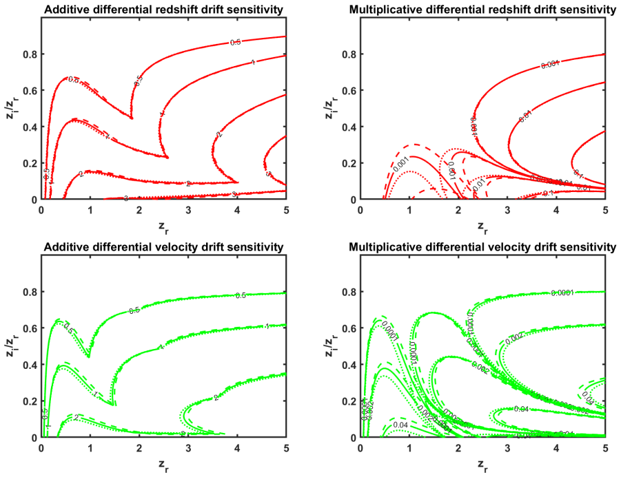
The carrying object is the dimensionless redshift drift $S_z = h[1+z-E(z)]$, with the corresponding spectroscopic velocity $S_v = (cH_0\Delta t)[1-E(z)/(1+z)]$, evaluated in a curved $w_0$CDM background. The forecast machinery is the Fisher matrix $F_{ij}=\sum_a (\partial f_a/\partial p_i)(1/\sigma_a^2)(\partial f_a/\partial p_j)$, whose inverse gives parameter covariances and whose determinant's inverse $n$th root defines the global figure of merit. The differential drift is modeled as the difference $S_z(z_r,z_i)=h[(z_r-z_i)-(E(z_r)-E(z_i))]$, and the paper's central comparison is between the theoretical sensitivity coefficients $\partial S/\partial p_i$ for the four parameters and across fiducial values $\Omega_k = -0.1, 0, +0.1$.
What would settle it
Measure, via end-to-end simulations of the differential drift reduction on the seven ANDES Golden Sample quasars, the achieved spectroscopic velocity uncertainty relative to the standard drift at intervening redshifts near $z_i/z_r\approx0.15$–$0.25$; if the typical ratio is $\gtrsim2$, the claimed $\sim15\%$ four-dimensional figure-of-merit gain from joint measurements does not materialize.
Extended reading notes
Core claim
On the paper's own terms, the central discovery is that spatial curvature is not a peripheral nuisance in redshift drift cosmology: it is a first-class parameter with sensitivity comparable to matter and greater than the dark energy equation of state. Working in a $w_0$CDM model with $E^2(z)=\Omega_k(1+z)^2+\Omega_m(1+z)^3+(1-\Omega_m-\Omega_k)(1+z)^{3(1+w_0)}$, the authors show that the drift's sensitivity coefficients to $\Omega_k$ and $\Omega_m$ behave similarly at low redshifts, and that the sensitivity to curvature is larger for closed than for open universes of the same $|\Omega_k|$. They then forecast, for the first time, joint standard and differential drift measurements on the seven Golden Sample quasars: with an intervening-to-reference redshift ratio around 0.15 and equal velocity uncertainties, the joint measurement improves the four-dimensional figure of merit by about 15% over standard drift plus priors, and the same data yield an indirect low-redshift measurement $S_v(z_i,0)=S_v(z_r,0)-S_v(z_r,z_i)$ that bridges the ELT and SKA redshift ranges.
Load-bearing premise
The joint-forecast gain assumes the differential redshift drift's per-target spectroscopic velocity uncertainty is proportional to the standard drift's—equal, twice, or four times worse—and the actual ratio has not been measured; if it is worse than about two, Figure 9 shows that most of the differential drift's figure-of-merit gain disappears.
Editorial extensions
If this is right
- SKA and ELT/ANDES redshift drift forecasts that assume flatness will overstate their constraining power, particularly for $\Omega_m$, because the strong $\Omega_m$–$\Omega_k$ anticorrelation weakens matter constraints when curvature is freed.
- A future drift detection at $z\approx1$ carries information about the sign of curvature: closed universes give a larger positive-drift window than open universes with the same $|\Omega_k|$, so the same measurement has different discriminating power in the two cases.
- Joint standard and differential drift measurements on the Golden Sample add roughly 15% to the four-parameter figure of merit at no extra telescope time, provided the differential drift velocity uncertainty is comparable to the standard one and the intervening redshift is low, $z_i/z_r\approx0.15$–$0.25$.
- Because $S_v(z_i,0)=S_v(z_r,0)-S_v(z_r,z_i)$, Golden Sample measurements can synthesize a prediction for low-redshift drift that the SKA can test directly; a mismatch, absent systematics, would indicate a breakdown of the cosmological principle.
- If the differential drift velocity uncertainty is a factor of two worse than the standard drift's, most of the joint-measurement gain disappears, so the main observing-strategy requirement is to keep the two uncertainties comparable.
Reading between the lines
- The authors do not pursue model selection, but the sign asymmetry implies that a single well-placed low-redshift drift detection could discriminate closed from open universes more cleanly than Gaussian parameter contours suggest.
- Their fixed-ratio assumption treats all seven quasars identically; allowing each line of sight its own intervening redshift would likely redistribute, and possibly increase, the reported joint gain.
- Because the differential measurement uses absorption features already in the same spectra, the joint analysis is best read as a data-analysis upgrade to an already planned observation rather than a new observing program.
- The assumed proportionality between differential and standard velocity uncertainties could be tested with existing high-resolution spectrograph data before the ELT era, giving an early empirical check on the forecast's main condition.
Editorial analysis
A structured set of objections, weighed in public.
Referee Report
Summary. The manuscript presents Fisher-matrix forecasts for standard and differential redshift drift measurements, allowing for a non-flat w0CDM background with free curvature Ωk. It derives analytic sensitivity coefficients from the Friedmann equation, reports that the sensitivity of the drift to curvature is comparable to that to matter and asymmetric between open and closed universes, and then produces forecasts for SKA and for the ELT ANDES Golden Sample. The paper's stated main novelty is a joint standard-plus-differential drift analysis for the Golden Sample (Section 5), which claims an additional up-to-15% figure-of-merit gain in the four-dimensional parameter space (Table 5).
Significance. The standard-drift forecasts with curvature are a useful and clearly presented extension of previous work, and the analytic sensitivity discussion is transparent and cross-checked with an independent code. The public availability of the Fisher code (FRIDDA) strengthens reproducibility. The open/closed asymmetry in sensitivities is an interesting qualitative result. However, the quantitative joint-measurement claim relies on observing geometries (zi/zr as low as 0.15) that are physically inaccessible for the Lyα-forest-based differential technique on the Golden Sample, which substantially limits the practical significance of the headline 15% gain.
major comments (1)
- [Section 5, Table 5 and Figure 9] The assumed range zi/zr ∈ [0.15,0.85] and the 'best case' zi/zr = 0.15 used to quote the maximal FoM gain in Table 5 are not physically realizable for the differential redshift drift technique as described in Section 4, which relies on the Lyman-α forest. For a Golden Sample quasar at zr, the lowest-redshift intervening absorber whose Lyα line falls in the observed spectrum is set by the blue cutoff of the forest; with a conservative 400 nm atmospheric/instrument cutoff for ANDES, zi_min ≈ 2.29, giving zi/zr ≈ 0.76 for the lowest-redshift quasar (zr = 3.0), and the ratio is only slightly lower (≈0.67) even if the Lyman limit at 91.2 nm is used. At the accessible ratios zi/zr ≳ 0.7, Figure 9 shows that the differential drift adds only a few percent to the FoM, so the reported 'additional 15%' is not observationally realizable. The authors should recompute the joint forecast for physically allowed geometries, or explicitly demonstrate an alternative absorption-line strategy that reaches low zi, and adjust the claims in Section 5 and the abstract accordingly.
minor comments (4)
- [Table 5 caption] The caption reads 'rounded off the the nearest integer'; this should be 'rounded off to the nearest integer'.
- [Figure 9] It would aid the reader if the physically allowed range of zi/zr (roughly ≳0.7) were marked on the figure, so that the falloff of the gain at accessible geometries is immediately visible.
- [Section 4, Eq. (10)-(12)] The text states that the definitions differ by a minus sign from [7,20] to recover the standard drift when zi = 0; it would be helpful to note explicitly that this sign choice also affects the sign of the plotted sensitivity coefficients, so that readers comparing with earlier work are not confused.
- [Section 6, Eq. (13)] The indirect measurement S_v(zi,0) = S_v(zr,0) − S_v(zr,zi) is correctly described as non-independent, but the text could state that its uncertainty is the quadrature sum of the two direct measurements, which is relevant for the proposed SKA consistency test.
Circularity Check
No significant circularity: the forecast chain is an analytic Fisher-matrix calculation from the Friedmann equation, with all simplifying assumptions stated rather than derived from the target results.
full rationale
The derivation chain is self-contained and not circular. The sensitivity coefficients in Section 2 are analytic derivatives of the dimensionless Hubble parameter E(z) from Eq. (5), and the curvature asymmetry is an explicit consequence of the stated parameterization, with the authors acknowledging in the Conclusions that a closed universe has more dark energy at fixed matter density. The forecasts in Section 3 use the standard Fisher-matrix definition, Eq. (7), with stated priors and the Golden Sample uncertainties taken from the external sample paper [17]; no parameter is fitted to the forecast outputs. The differential redshift drift is defined in Eqs. (10)-(12) as the difference of two standard drifts, and the joint forecast in Section 5 combines the standard and differential observables as independent Fisher information. The zi/zr range and the uncertainty proportionality factors are explicitly described as simplifying assumptions, not as predictions or as consequences of the results. The self-cited FRIDDA code [19] is said to be "further validated by a second independent code (written in Matlab instead of Python)", so the self-citation is not load-bearing and the forecasts do not reduce to prior work. The separate feasibility concern raised by the reviewer, namely that the Golden Sample Ly-alpha forest may not allow zi/zr values as low as 0.15, is an observational realism caveat about the assumed range, not a circular reduction of the forecast to its inputs. Overall, the paper's conclusions follow from its stated equations, assumptions, and external inputs, with no circular step.
Assumptions & free parameters
free parameters (6)
- fiducial Hubble parameter h =
0.7
- fiducial matter density Omega_m =
0.3
- fiducial dark energy equation of state w0 =
-1
- fiducial curvature Omega_k =
0, +0.1, -0.1
- prior widths sigma(h), sigma(Omega_m), sigma(w0), sigma(Omega_k) =
0.1, 0.05, 0.15, 0.2
- differential drift uncertainty ratio =
1x, 2x, 4x standard
assumptions (7)
- domain assumption Friedmann equation for a w0CDM model with curvature, Eq. 5
- standard math Redshift drift formula Delta z / Delta t = H0 [1 + z - E(z)], Eq. 1
- standard math Fisher matrix formalism with Gaussian likelihood, Eqs. 7-9
- domain assumption No radiation component for z <= 5
- domain assumption Homogeneous and isotropic FRW background
- domain assumption SKA and ELT Golden Sample noise models from [8] and [17]
- ad hoc to paper Differential drift uncertainty is proportional to standard drift uncertainty
Cite this review
Pith. "Pith review of Impact of spatial curvature on forecast constraints from standard and differential redshift drift measurements." pith.science (2026). https://pith.science/paper/MW2RZEHI
@misc{pith2026241207532,
  author       = {Pith},
  title        = {Pith review of: Impact of spatial curvature on forecast constraints from standard and differential redshift drift measurements},
  year         = {2026},
  howpublished = {\url{https://pith.science/paper/MW2RZEHI}},
  note         = {Machine review of arXiv:2412.07532}
}
abstract
The redshift drift of objects following the cosmological expansion is a unique model-independent probe of background cosmology, detectable by astrophysical facilities presently under construction. Previous forecasts for such measurements assume flat universes. We explore the impact of relaxing this assumption on the constraining power of the redshift drift, focusing on the two most promising routes for its measurement: the SKA at low redshifts, and the Golden Sample for the ELT's ANDES spectrograph at higher redshifts. We also discuss the cosmological sensitivity of possible differential redshift drift measurements, both on their own and, for the specific case of the Golden Sample, in combination with the standard method. Overall, we find that the sensitivity of the redshift drift to curvature is comparable to that of matter (especially at low redshifts) and higher than the sensitivity to the dark energy equation of state. We also show that the sensitivity of redshift drift measurements to these cosmological parameters is asymmetric with respect to the curvature parameter, being different for open and closed universes with the same absolute value of the curvature parameter $\Omega_k$.
Figures


Figures from the paper (7 more)




Reference graph
Works this paper leans on
-
[1]
A. Sandage, The Change of Redshift and Apparent Luminosity of Galaxies due to the Deceleration of Selected Expanding Universes., Astrophys. J. 136 (1962) 319
work page 1962
-
[2]
Liske, et al., Cosmic dynamics in the era of Ex- tremely Large Telescopes, Mon
J. Liske, et al., Cosmic dynamics in the era of Ex- tremely Large Telescopes, Mon. Not. Roy. Astron. Soc. 386 (2008) 1192–1218
work page 2008
-
[3]
J.-P. Uzan, C. Clarkson, G. F. R. Ellis, Time drift of cosmological redshifts as a test of the Copernican principle, Phys. Rev. Lett. 100 (2008) 191303
work page 2008
-
[4]
C. Quercellini, L. Amendola, A. Balbi, P. Cabella, M. Quartin, Real-time Cosmology, Phys. Rept. 521 (2012) 95–134
work page 2012
-
[5]
Heinesen, Redshift drift as a model indepen- dent probe of dark energy, Phys
A. Heinesen, Redshift drift as a model indepen- dent probe of dark energy, Phys. Rev. D 103 (2021) L081302
work page 2021
-
[6]
Darling, Toward a Direct Measurement of the Cosmic Acceleration, Astrophys
J. Darling, Toward a Direct Measurement of the Cosmic Acceleration, Astrophys. J. 761 (2012) L26
work page 2012
-
[7]
Cooke, The ACCELERATION programme: I
R. Cooke, The ACCELERATION programme: I. Cosmology with the redshift drift, Mon. Not. Roy. Astron. Soc. 492 (2020) 2044–2057
work page 2020
-
[8]
H.-R. Kl ¨ockner, D. Obreschkow, C. Martins, A. Raccanelli, D. Champion, A. L. Roy, A. Lobanov, J. Wagner, R. Keller, Real time cosmology - A direct measure of the expansion rate of the Universe with the SKA, PoS AASKA14 (2015) 027
work page 2015
Show all 21 references
-
[9]
Liske, et al., Top Level Requirements For ELT- HIRES, Technical Report, Document ESO 204697 Version 1, 2014
J. Liske, et al., Top Level Requirements For ELT- HIRES, Technical Report, Document ESO 204697 Version 1, 2014
2014
-
[10]
C. J. A. P. Martins, et al., Cosmology and funda- mental physics with the ELT-ANDES spectrograph, Exper. Astron. 57 (2024) 5
2024
-
[11]
C. S. Alves, A. C. O. Leite, C. J. A. P. Martins, J. G. B. Matos, T. A. Silva, Forecasts of redshift drift constraints on cosmological parameters, Mon. Not. Roy. Astron. Soc. 488 (2019) 3607–3624
2019
-
[12]
B. A. R. Rocha, C. J. A. P. Martins, Redshift drift cosmography with ELT and SKAO measurements, Mon. Not. Roy. Astron. Soc. 518 (2022) 2853–2869
2022
-
[13]
C. M. J. Marques, C. J. A. P. Martins, B. G. L ´opez, Watching the Universe’s acceleration era with the SKAO, Mon. Not. Roy. Astron. Soc. 527 (2023) 9918–9929
2023
-
[14]
Balbi, C
A. Balbi, C. Quercellini, The time evolution of cos- mological redshift as a test of dark energy, Mon. Not. Roy. Astron. Soc. 382 (2007) 1623–1629
2007
-
[15]
Aghanim, et al., Planck 2018 results
N. Aghanim, et al., Planck 2018 results. VI. Cosmo- logical parameters, Astron. Astrophys. 641 (2020) A6. [Erratum: Astron.Astrophys. 652, C4 (2021)]
2020
-
[16]
Di Valentino, A
E. Di Valentino, A. Melchiorri, J. Silk, Planck evi- dence for a closed Universe and a possible crisis for cosmology, Nature Astron. 4 (2019) 196–203
2019
-
[17]
Cristiani, et al., Spectroscopy of QUBRICS quasar candidates: 1672 new redshifts and a golden sample for the Sandage test of the redshift drift, Mon
S. Cristiani, et al., Spectroscopy of QUBRICS quasar candidates: 1672 new redshifts and a golden sample for the Sandage test of the redshift drift, Mon. Not. Roy. Astron. Soc. 522 (2023) 2019–2028
2023
-
[18]
C. Dong, A. Gonzalez, S. Eikenberry, S. Jeram, M. Likamonsavad, J. Liske, D. Stelter, A. Townsend, Forecasting cosmic acceleration measurements us- ing the Lyman-α forest, Mon. Not. Roy. Astron. Soc. 514 (2022) 5493–5505
2022
-
[19]
C. M. J. Marques, C. J. A. P. Martins, C. S. Alves, FRIDDA: Fisher foRecast code for combIned reD- shift Drift and Alpha, Astrophysics Source Code Li- brary, record ascl:2305.001, 2023
2023
-
[20]
Esteves, C
J. Esteves, C. J. A. P. Martins, B. G. Pereira, C. S. Alves, Cosmological impact of redshift drift mea- surements, Mon. Not. Roy. Astron. Soc. 508 (2021) L53–L57
2021
-
[21]
P. K. Aluri, et al., Is the observable Universe consis- tent with the cosmological principle?, Class. Quant. Grav. 40 (2023) 094001. 19
2023
Reviewed August 11, 2026 · model on record in the stance chip above.
Discussion (0). Continue with ORCID to comment.