REVIEW 2 major objections 5 minor 10 references
On the resolution of dual readout calorimeters
T0 review · 2 major / 5 minor · reviewed 2026-08-10 · deepseek-v4-flash
Pith's one-line read One resolution formula predicts when the dual-readout correction improves hadronic calorimeters and when it hurts them.
desk verdict A clean, honest derivation of a dual-readout resolution formula, validated broadly; the covariance check the stress-test wants would be nice but the paper already earns a serious review. read the letter →
The pith
A machine-rendered reading of the paper's core claim, the machinery that carries it, and where it could break.
The reading
What carries the argument
The load-bearing object is the corrected estimator $D$, a linear projection of the $(C,S)$ pair along their correlation line onto the electron energy scale. The argument uses simple error propagation: because the scintillation and Cherenkov signals both depend on the same electromagnetic fraction $f$, their covariance is $(1-h_S)(1-h_C)\sigma_f^2$; inserting this covariance into the standard error-propagation formula gives Eq. (11). The secondary machinery is the decomposition of the shower into an electromagnetic part, a non-electromagnetic part, and the loss fractions $f_{NC}$ (nuclear binding) and $f_{ES}$ (escaping energy), which yields approximate formulas for $h_S$ and $\sigma_S$ and makes the meaning of the correction concrete.
What would settle it
Run a full shower simulation, compute the energy estimates $S$ and $C$ shower by shower, and measure their covariance directly; the formula requires $\mathrm{cov}(S,C) = (1-h_S)(1-h_C)\sigma_f^2$, so a disagreement larger than the statistical uncertainties would invalidate the error-propagation chain that produces Eq. (11).
Extended reading notes
Core claim
The paper's central claim is Eq. (11): $$\sigma_D = \frac{1}{h_S-h_C}\sqrt{(1-h_C)^2\$sigma_S^{2}$ + (1-h_S)^2\$sigma_C^{2}$ - 2(1-h_S)^2(1-h_C)^2\$sigma_f^{2}$},$$ which predicts the resolution of the dual-readout-corrected energy estimate $D=\frac{(1-h_C)S-(1-h_S)C}{h_S-h_C}$ for hadrons of fixed energy. Here $h_S$ and $h_C$ are the average responses of the scintillation and Cherenkov readouts to the non-electromagnetic part of the shower, and $\sigma_f$ is the rms fluctuation of the electromagnetic fraction. The paper tests this expression against simulated showers in a homogeneous crystal calorimeter, two fiber calorimeters, and two sampling-tile calorimeters, finding predicted corrected resolutions close to the simulated values for all five geometries, including the SampS case where the correction degrades resolution because escaping energy and large correlated fluctuations dominate. The same derivation shows the correction compensates not only for nuclear binding-energy loss but also for energy escaping the calorimeter and energy missed by the clustering algorithm, and it yields approximate formulas for $h_S$ and $\sigma_S$ in terms of sampling fractions and the loss fractions $f_{NC}$ and $f_{ES}$.
Load-bearing premise
The formula assumes that the electromagnetic fraction $f$ of the shower is roughly Gaussian with moderate width and that $h_S$ and $h_C$ are constants independent of $f$ and of the noise terms; where those assumptions break down, as in the small SampS calorimeter, the quantitative agreement loosens even though the formula still describes the trend.
Editorial extensions
If this is right
- With measured or estimated $h_S$, $h_C$, $\sigma_S$, $\sigma_C$, and $\sigma_f$, Eq. (11) predicts before full construction whether the dual-readout correction will improve a proposed calorimeter's hadronic resolution.
- The correction is expected to hurt when the Cherenkov readout is noisy: Eq. (13) states that the dual-readout estimate is worse than the scintillation-only estimate unless $\sigma_f > \sigma_C/(\sqrt{2}(1-h_C))$.
- Dual-readout compensation applies to scale fluctuations from escaping energy and clustering losses as well as from nuclear binding energy, so containment and algorithm efficiency enter the resolution budget explicitly.
- For nearly compensating geometries such as Fiber2, the dual-readout correction gives only a modest improvement because the scintillation response already has little dependence on $f$.
- The formula explains the counterintuitive SampS result from an earlier simulation, predicting the observed worsening of resolution for a small, poorly contained calorimeter.
Reading between the lines
- A practical consequence not spelled out in the paper: Eq. (13) can be used as a go/no-go test during design, comparing expected Cherenkov noise to the electromagnetic-fraction fluctuation before investing in the second readout.
- The same covariance argument transfers to any two-readout estimator that shares a common latent variable: whenever the correlated fluctuation term is small compared with the uncorrelated noises, the corrective linear combination will degrade rather than improve resolution.
- The formula suggests a direct simulation diagnostic: measure the empirical shower-by-shower covariance of $S$ and $C$ and compare it with $(1-h_S)(1-h_C)\sigma_f^2$; a large discrepancy would identify correlations beyond the simple Gaussian-$f$ model.
- For future collider calorimeters, the explicit appearance of $f_{ES}$ in $h_S$ turns containment into a quantitative resolution input, so optimizing length and transverse size becomes an optimization of the resolution formula itself.
Editorial analysis
A structured set of objections, weighed in public.
Referee Report
Summary. The paper derives a closed-form expression for the energy resolution of a dual-readout calorimeter after the dual-readout correction, Eq. (11), starting from the ansatz that the scintillation and Cherenkov signals share a common dependence on the electromagnetic fraction f, plus independent noise terms. The covariance between S and C is computed in Appendix A, giving cov(S,C) = (1-hS)(1-hC)σf². The formula is tested against a toy Monte Carlo and against GEANT4 simulations of five calorimeter geometries (PbWO, fiber, and sampling calorimeters), with the predicted corrected resolution compared in Table 6. The paper also presents approximate formulae for hS and σS in terms of binding-energy loss, escaping energy, and sampling-fraction fluctuations. The stated purpose is to explain when the dual-readout correction improves or worsens the resolution.
Significance. If the formula is reliable, it provides a simple, design-oriented tool for estimating the performance of dual-readout calorimeters without full simulation, and it clarifies the counterintuitive result reported in Ref. [4] that the correction can degrade resolution. The paper is explicitly pedagogical and is likely to be useful to newcomers to the field. The full GEANT4 comparison across five geometries, including one (SampS) where the correction worsens resolution, is a valuable stress test. The toy simulation code is made publicly available on GitHub, and the derivation in Appendix A is algebraically correct. The main weaknesses are an incorrect inequality in one of the derived conditions, and a verification that tests the covariance model only indirectly through the final σD.
major comments (2)
- [Sec. 2, Eq. (14)] The inequality in Eq. (14) is reversed. Starting from Eq. (11), σD > σS is equivalent to σf² < [(2−χ)σS²] / [2(1−hC)(1−hS)] + σC² / [2(1−hC)²], not the '>' condition printed. For a concrete counterexample with hS=0.9, hC=0.6, σS=σC=0.05, and σf=0.3, the RHS of Eq. (14) is 0.0625 while σf²=0.09, so the printed condition says σD > σS, but Eq. (11) gives σD≈0.039 < σS=0.05. The accompanying discussion near Eq. (13) should be re-examined as well, since the condition for the sum of the second and third terms in Eq. (12) to be positive depends on the same inequality direction.
- [Sec. 4.4, Table 6] The verification of Eq. (11) against the full simulation is indirect: hS, hC, and σf are all extracted from the same simulated events used to measure σD, and the comparison only checks the final σD. Since the only non-trivial input of Eq. (11) beyond the measured σS and σC is the covariance model of Eq. (10), a direct comparison between the model covariance (1−hS)(1−hC)σf² and the covariance computed from the simulated (S,C) pairs would provide a much more sensitive test of the central assumption. The statement in Sec. 4.3 that correlations between fNC and fES 'do not affect the prediction' of the corrected resolution is not demonstrated; reporting a direct covariance comparison, or at least a quantitative estimate of the neglected contributions, would substantially strengthen the verification claim.
minor comments (5)
- [Sec. 2, Eq. (6)] The partial derivatives in Eq. (6) are written as ∂E/∂S and ∂E/∂C, but the quantity being propagated is D; this should be ∂D/∂S and ∂D/∂C.
- [Sec. 4.4, Eq. (31)] Equation (31) contains a typographical error: the term (1−<S)2 is missing the closing angle bracket, and the overall layout makes the placement of the denominator ambiguous; please reformat.
- [Sec. 4.2, Eq. (20)] The definition fNC = (EB − EES − EI)/EB normalizes the binding-energy loss to the total beam energy, but in Eqs. (19), (22), and (24) the same symbol is used as a fractional loss of the non-EM component. Please clarify the intended normalization and reconcile it with the caption of Fig. 15, which refers to division by the non-EM energy.
- [Table 5] In the Fiber2 row, σf is listed as 0.12 ± 0.1; the uncertainty appears to be a factor of 10 too large and is inconsistent with the other entries; likely ±0.01 is intended.
- [General] There are several typographical errors, including 'simulatate' in Sec. 4.1, 'the the D resolution' in Sec. 3, 'ansantz' in Sec. 4.2, and the use of 'fN C' and 'fESC' with inconsistent spacing; a careful proofread is recommended.
Circularity Check
No significant circularity: the central resolution formula is independently tested against GEANT4; only the toy-MC check is a closed algebraic loop.
-
self definitional
[Section 3, 'Tests with a toy simulation']
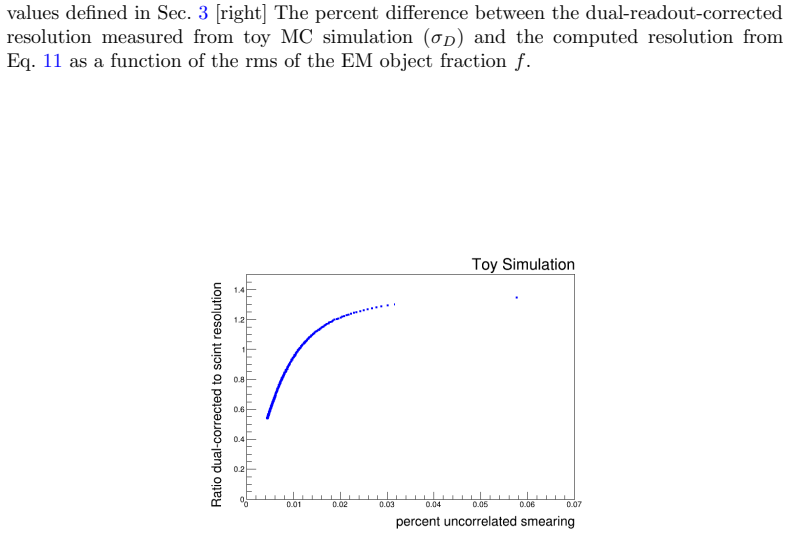
"We used a toy Monte Carlo simulation [5] to test Eq. 11. The toy models f as a Gaussian. The S and C signals are calculated from f using Eqs. 1 and 2. The S and C signals are then smeared using separate Gaussians to simulate sources of resolution uncorrelated between the two."
Eq. 11 is derived in Sec. 2 by propagating errors through exactly Eqs. 1 and 2, with f Gaussian and independent noise terms x2, x3. The toy simulation generates S and C from those same equations and Gaussian smearing, so the measured toy sigma_D is the same quantity that Eq. 11 computes analytically. The agreement is therefore guaranteed by construction up to Monte Carlo statistics; the toy is a check of the algebra, not an empirical test of the physical ansatz. This loop is not load-bearing because the paper also compares Eq. 11 against independent GEANT4 full simulation results in Sec. 4.4, where the parameters are measured from simulated showers rather than generated from the formula.
full rationale
The central claim of the paper is the closed-form resolution formula Eq. 11, obtained by error propagation from the ansatz Eqs. 1-2 with the covariance cov(S,C) = (1-hS)(1-hC)sigma_f^2. The derivation itself is a standard mathematical calculation, not a fit. The toy simulation in Sec. 3 is self-referential: it generates S and C from the same equations used to derive Eq. 11, so it can only verify algebraic consistency. However, the full GEANT4 simulations in Sec. 4 provide an independent test: the calorimeter response is simulated from particle physics, not from Eqs. 1-2, and the inputs hS, hC, sigma_f, sigma_S, sigma_C are extracted from the simulated distributions. Table 6 then compares the predicted and measured sigma_D for five different calorimeter geometries, including a case (SampS) where the correction worsens resolution; this is a falsifiable, non-tautological check. The paper explicitly acknowledges the conditions under which the ansatz is violated (Sec. 4.3, e.g., strong fNC-fES correlation for SampS), and those caveats concern model accuracy rather than circularity. Self-citations to Refs. [3] and [4] are not load-bearing: the relevant SampS and Fiber1 results are re-simulated and quoted directly in this paper. Overall, the derivation is self-contained and the central verification is independent, with only the toy-MC closure and a mild sharing of simulated inputs preventing a fully clean bill of health.
Assumptions & free parameters
free parameters (5)
- hS (average non-EM scintillation response) =
0.740 (PbWO), 1.192 (Fiber1), 1.075 (Fiber2), 1.29 (SampL), 0.45 (SampS)
- hC (average non-EM Cherenkov response) =
0.006 (PbWO), 0.21 (Fiber1), 0.14 (Fiber2), 0.08 (SampL), 0.04 (SampS)
- σf and <f> (EM fraction fluctuation and mean) =
Per calorimeter: σf 0.086-0.15, <f> 0.503-0.669 (Tables 4-5)
- g1, g2 (EM/non-EM sampling fraction ratios) =
Per calorimeter, Table 3; e.g., Fiber1 g2 = 2.09 ± 0.06
- σg/g (sampling fraction fluctuation) =
Per calorimeter, Table 8 (e.g., Fiber1 0.0515)
assumptions (4)
- domain assumption The dual-readout response is linear in the electromagnetic fraction f: S = E(f + (1−f)hS) and C = E(f + (1−f)hC) with constant hS, hC (Eqs. 1-2).
- domain assumption f is Gaussian-distributed with moderate width.
- domain assumption Noise terms in S and C are mutually independent and independent of f.
- ad hoc to paper The ansatz S = g1 fγπ EB + g2[(1−fRπ)EB − (1−fRγ)fγπ EB](1−fNC−fES) (Eq. 19)
Cite this review
Pith. "Pith review of On the resolution of dual readout calorimeters." pith.science (2026). https://pith.science/paper/NL5UNWIL
@misc{pith2026250115329,
  author       = {Pith},
  title        = {Pith review of: On the resolution of dual readout calorimeters},
  year         = {2026},
  howpublished = {\url{https://pith.science/paper/NL5UNWIL}},
  note         = {Machine review of arXiv:2501.15329}
}
read the original abstract
Dual readout calorimeters allow state-of-the-art resolutions for hadronic energy measurements. Their various incarnations are leading candidates for the calorimeter systems for future colliders. In this paper, we present a simple formula for the resolution of a dual readout calorimeter, which we verify with a toy simulation and with full simulation results. This formula can help those new to dual readout calorimetry understand its strengths and limitations. The paper also highlights that the dual readout correction works not just to compensate for binding energy loss, but also for energies escaping the calorimeter or clustering algorithm. Formulae are also presented for approximate resolutions and energy scales in terms of different sources of response.
Figures


Figures from the paper (15 more)


Reference graph
Works this paper leans on
-
[4]
S. Chekanov, S. Eno, S. Magill, C. Palmer, L. Wu, M. Aamir, Geant4 simulations of sampling and homogeneous hadronic calorimeters with dual readout for future colliders, ”Nucl. Instrum. Meth. A” 1072 (2025) 170200. doi:https://doi.org/10.1016/j..2025.170200
-
[1]
S. Lee, M. Livan, R. Wigmans, Dual-readout calorimetry, Rev. Mod. Phys. 90 (2) (2018) 025002. arXiv:1712.05494, doi:10.1103/ RevModPhys.90.025002
arXiv 2018
-
[2]
R. Aly, et al., First test-beam results obtained with IDEA, a detector concept designed for future lepton colliders, Nucl. Instrum. Meth. A 958 (2020) 162088, proceedings of the Vienna Conference on Instrumenta- tion 2019. doi:https://doi.org/10.1016/j.nima.2019.04.042
-
[3]
M. T. Lucchini, C. G. Tully, W. Chung, S. C. Eno, Y. Lai, L. Lucchini, M.-T. Nguyen, New perspectives on segmented crystal calorimeters for future colliders, JINST 15 (11) (2020) P11005.arXiv:2008.00338, doi: 10.1088/1748-0221/15/11/P11005
arXiv 2020
-
[5]
URL https://github.com/saraheno/DualReadoutToy
github repository for toy (2024). URL https://github.com/saraheno/DualReadoutToy
work page 2024
-
[6]
Agostinelli, et al., GEANT4 – a simulation toolkit, Nucl
S. Agostinelli, et al., GEANT4 – a simulation toolkit, Nucl. Instrum. Meth. A 506 (2003) 250–303. doi:10.1016/S0168-9002(03)01368-8
-
[7]
URL https://dd4hep.web.cern.ch/dd4hep/
Detector description toolkit for high energy physics (2024). URL https://dd4hep.web.cern.ch/dd4hep/
work page 2024
-
[8]
Abdullin, et al., Design, performance, and calibration of CMS hadron- barrel calorimeter wedges, Eur
S. Abdullin, et al., Design, performance, and calibration of CMS hadron- barrel calorimeter wedges, Eur. Phys. J. C 55 (2008) 159. doi:10.1140/ epjc/s10052-008-0573-y
work page 2008
Show all 10 references
-
[9]
Bedeschi, A detector concept proposal for a circular e+e− collider, PoS ICHEP2020 (2021) 819
F. Bedeschi, A detector concept proposal for a circular e+e− collider, PoS ICHEP2020 (2021) 819. doi:10.22323/1.390.0819
2021 doi
-
[10]
J. B. Birks, The theory and practice of scintillation counting, Interna- tional Series of Monographs on Electronics and Instrumentation, Vol- ume 27, Pergamon Press, The Macmillan Company, New York, 1964. doi:10.1016/C2013-0-01791-4 . 30 Appendix A. Derivation of the Covarianc...
1964 doi
Reviewed August 10, 2026 · model on record in the stance chip above.
Discussion (0). Continue with ORCID to comment.