REVIEW 3 major objections 6 minor 46 references
Learning Backward Transport for Source Localization
T0 review · 3 major / 6 minor · reviewed 2026-07-30 · grok-4.5
Pith's one-line read Learning the backward transport of tracers turns source finding into sampling, and classical search behaviors fall out of one drift.
desk verdict Clean physics-first unification of surge/cast/chemotaxis via a learned backward propagator; solid enough to referee, with the Gaussian approximation as the main open check. read the letter →
The pith
A machine-rendered reading of the paper's core claim, the machinery that carries it, and where it could break.
The reading
What carries the argument
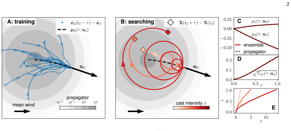
The inverse-Fokker–Planck drift family (Eq. 7): given the Gaussian superposition F of backward propagators, the drift that makes the agent’s law track F decomposes into transport of the mean (surge), score ascent corrected for spreading uncertainty (chemotaxis), and an antisymmetric gauge Ψ that generates casting along level sets.
What would settle it
Train the same Gaussian propagator, run the backtracking agents and the best-tuned cast-and-surge or spiral baselines in the same 2D turbulent concentration fields, and check whether backtracking still yields shorter successful trajectories at equal or lower lost fraction across the three wind regimes; failure of that trade-off curve, or large mismatch between agent ensemble moments and propagator moments, would refute the claim.
Extended reading notes
Core claim
Source localization from sparse chemical detections can be framed as a Schrödinger bridge between plausible emission positions and detection points, using a learned backward propagator of passive tracers. Sampling that bridge via the inverse-Fokker–Planck drift family makes classical chemotaxis and cast-and-surge complementary facets of one transport-based dynamics, and a single Galilean-invariant learned propagator outperforms tuned classical strategies across wind regimes in two-dimensional turbulence.
Load-bearing premise
The true backward transport of tracers in turbulence can be replaced by a simple isotropic Gaussian whose few scalar coefficients are fit by a small neural net, so the closed-form probability map and derived drift stay faithful.
Editorial extensions
If this is right
- One offline-learned, Galilean-invariant propagator can be reused under arbitrary mean wind without retraining.
- Cast intensity Ψ and diffusion D become explicit knobs trading geodesic surge against exploratory casting inside a single dynamics.
- In pure diffusion with multi-detection memory the same drift statistically aligns with the concentration gradient, recovering chemotaxis.
- The framework extends in principle to moving sources and to any setting where transport statistics can be learned offline and inverted from local observations.
Reading between the lines
- If the Gaussian approximation is the load-bearing limit, score-based or normalizing-flow propagators could extend the same sampling picture to strongly non-Gaussian or multi-point transport without changing the drift logic.
- The same backward-propagator sampling could be tried on network diffusion or epidemic source inference, where an offline-learned reverse kernel plays the role of the fluid propagator.
- Task-optimizing Ψ and D online, rather than fixing a casting schedule, is a direct next experiment the paper’s gauge freedom already licenses.
Editorial analysis
A structured set of objections, weighed in public.
Referee Report
Summary. The manuscript proposes source localization in a flow by learning the backward propagator of passive tracers offline and, upon each detection, sampling candidate emission locations with Langevin dynamics whose drift is obtained by inverting the Fokker–Planck equation for a superposition of those propagators (Eqs. 4–7). Classical chemotaxis and cast-and-surge are recovered as complementary pieces of that single drift (mean transport, score ascent, and a divergence-free casting gauge Ψ). In statistically steady 2D inverse-cascade turbulence the method, using one Galilean-invariant Gaussian propagator trained at zero mean wind, produces a favorable mean-length versus lost-fraction trade-off against tuned cast-and-surge and Archimedean-spiral baselines across isotropic, moderate, and strong wind; a pure-diffusion limit is shown analytically and numerically to align with chemotaxis when multiple detections are retained.
Significance. If the results hold, the work offers a physically grounded alternative to heuristic and black-box RL search policies: strategies emerge from a learned transport model rather than from direct policy optimization, with explicit Galilean transfer across wind regimes and a transparent drift decomposition. Strengths include the closed-form inverse-Fokker–Planck family (7), ensemble validation that agent statistics track the propagator (Fig. 1c–d), the pure-diffusion alignment derivation (9), and a single offline propagator reused without retraining. That combination of interpretability, transferability, and competitive performance is of clear interest for olfactory search, environmental monitoring, and related inverse transport problems.
major comments (3)
- [After Eq. (2); End Matter; Fig. 1, 3] Text after Eq. (2) and End Matter: the central claims rest on replacing the true backward kernel by a low-parameter isotropic Gaussian (scalars α_d, β_d, γ_d fit by a small MLP). In 2D inverse-cascade turbulence, single-particle backward densities can develop non-Gaussian tails and vortex-induced structure; a mean/covariance match need not place probability mass correctly. Fig. 1(c–d) only checks that agents reproduce the fitted Gaussian’s μ and Σ, not that the Gaussian matches the empirical tracer law. Please add a quantitative fidelity check on held-out tracers (e.g. held-out log-likelihood, KL or Wasserstein to a nonparametric/histogram estimate, or tail-quantile errors) and state whether residual non-Gaussianity is small relative to the performance margins in Fig. 3. Without this, it remains unclear whether outperformance traces to faithful transport learning or to the drift structur
- [Eq. (4); footnote 38; turbulence results (M=1)] Eq. (4) and the M=1 turbulence results: detections are assumed conditionally independent so that intensity-weighted log-propagators superpose into a single Gaussian F. In a persistent turbulent plume, successive detections along one trajectory are correlated through the same coherent structures. The paper reports robust performance with M=1 and attributes it to directional information in the flow, but does not test whether violating independence (or using a weighted mixture instead of the log-superposition noted in footnote 38) changes the Pareto front in Fig. 3. A short ablation—M>1 with the same propagator, or a mixture vs log-sum comparison—would show that the reported gains are not an artifact of the independence closure.
- [Fig. 3; performance comparison paragraph] Fig. 3 and baseline protocol: backtracking is swept over casting intensity ψ and compared to cast-and-surge (cone aperture and surge duration) and Archimedean spirals (branch spacing), with baselines tuned to minimize lost fraction. The comparison would be more convincing if the same information set were equalized: classical cast-and-surge as implemented typically does not use the local velocity fluctuation u_d that conditions the learned propagator, nor the same detection memory. Please state explicitly what observables each baseline receives and, if baselines are denied u_d, either grant them an equivalent wind cue or discuss that part of the gain may come from velocity conditioning rather than from the Schrödinger-bridge construction per se.
minor comments (6)
- [Eq. (8)] Eq. (8) couples physical time t to backtracking lag τ by imposing constant speed |dX/dt|=U. This is natural for comparison to heuristics but is a strong restriction; a brief remark on how results change if τ=t or if speed is allowed to vary with |b| would clarify robustness of the Pareto curves.
- [Fig. 2] Fig. 2: only subsets of the domain are shown and the concentration field is the initial snapshot; a sentence on whether the field is frozen or live during search, and on the relative scale of ℓ_0 to the integral scale, would help readers interpret trajectory geometry.
- [End Matter (chemotactic tests)] End Matter, chemotaxis tests: mean trajectory length scaling as 1/√Δt for stochastic paths is noted; consider reporting arrival time or a Δt-independent path functional so that panel 4(b) is comparable to the constant-speed turbulence metrics.
- [Eq. (2); Eq. (A1)] Notation: τ is both the backtracking lag and, in places, a dummy integration variable in the Feynman–Kac formula (A1); a consistent distinction would avoid confusion with physical time t.
- [After Eq. (7)] The gauge choice Ψ_12 = ψ U σ/(s+σ) is described as minimal; one sentence on alternatives tried (or why this form) would aid reproducibility.
- [Fig. 3; abstract] Typos/style: “trajecotry” in Fig. 3(a) y-axis; “Schr¨ odinger” spacing is inconsistent in the abstract vs body; arXiv stamp and dated “July 30, 2026” should be cleaned for journal submission.
Circularity Check
No load-bearing circularity: offline tracer fit, inverse-FP drift, and search metrics are independent; only minor free-parameter tuning of casting intensity.
-
other
[Eq. (7)–(8) and Fig. 3(a); text on casting intensity ψ]
"Here, we define it by comparing the agent's visual range s with a measure of spatial uncertainty, σ=[Tr(Σ−1)]−1/2 ... Ψ12=ψUσ/(s+σ) with U a reference speed and ψ the dimensionless casting intensity. ... the family of backtracking strategies obtained by varying ψ generates a continuous trade-off in the plane of mean trajectory length versus lost fraction"
ψ and the constant-speed coupling (8) are free design choices, not derived from first principles; varying them produces the Pareto curves used to claim superiority over tuned baselines. This is ordinary hyperparameter exploration (baselines are likewise tuned on cone aperture/spiral spacing), not a fitted quantity renamed as an independent prediction. Flagged only as residual softness, not load-bearing circularity.
full rationale
The derivation chain is self-contained and not circular in the sense of this pass. The backward propagator is fit offline by maximum likelihood to an independent ensemble of passive-tracer trajectories (End Matter), not to search success. Source localization is then recast as sampling the resulting map F via a Langevin dynamics whose drift is obtained by solving the inverse Fokker–Planck problem so that the agent density tracks F; that construction is mathematical, not a fit-to-target. Classical surge, cast, and chemotaxis are identified with distinct terms in the closed-form drift family (Eq. 7), which is an interpretive decomposition rather than insertion of those behaviors as training targets. Empirical outperformance (Fig. 3) is measured on concentration fields under transferred mean winds without refitting the propagator to the success metric. Self-citations (e.g. [39] for the gauge form of drifts) supply a technical tool and are not used as uniqueness theorems that force the central claim. The only residual softness is that the casting intensity ψ and the constant-speed map (8) are free behavioral choices varied to trace the reported length-vs-lost trade-off—analogous to baseline hyperparameter sweeps, not a fitted input renamed as prediction. Score 1 reflects that minor free-parameter role; the central physics-to-strategy chain does not reduce to its inputs by construction.
Assumptions & free parameters
free parameters (6)
- casting intensity ψ =
order-1 values; figures show range including ~1–5
- MLP weights for α_d, β_d, γ_d =
not reported numerically
- detection threshold θ* =
1.33
- visual range s and agent size a =
s=10a, a=Δx
- agent diffusivity ε (chemotaxis tests) =
1e-3
- max trajectory length cutoff =
2×10^4 a
assumptions (6)
- domain assumption Concentration at a point is determined by backward Lagrangian tracer trajectories (Feynman–Kac / passive-scalar duality).
- standard math Agent position density tracks F iff the drift satisfies the inverse Fokker–Planck relation (6)–(7), including arbitrary antisymmetric Ψ.
- ad hoc to paper Detections are conditionally independent so log-propagators may be intensity-weighted and superposed into a single Gaussian F (Eq. 4).
- domain assumption Turbulent fluctuations are statistically homogeneous and isotropic enough that μ and Σ are isotropic tensor functions of u_d only.
- ad hoc to paper A single-point conditional Gaussian propagator learned from any passive tracer adequately replaces the exact path-functional backward kernel G for search.
- ad hoc to paper Physical time and backtracking lag are coupled by constant agent speed |dX/dt|=U via Eq. (8) when comparing to classical heuristics.
invented entities (1)
-
Family of backtracking drifts (Eq. 7) with casting gauge Ψ ∝ ψ U σ/(s+σ)
Cite this review
Pith. "Pith review of Learning Backward Transport for Source Localization." pith.science (2026). https://pith.science/paper/OPVEBYIU
@misc{pith2026260726892,
  author       = {Pith},
  title        = {Pith review of: Learning Backward Transport for Source Localization},
  year         = {2026},
  howpublished = {\url{https://pith.science/paper/OPVEBYIU}},
  note         = {Machine review of arXiv:2607.26892}
}
read the original abstract
We address the problem of locating a chemical source in a flow. Based on the duality between the concentration field and Lagrangian tracer trajectories, we interpret concentration detections as evidence of paths connecting the source to the detection points. This Schr\"odinger bridge formulation between plausible emission positions and detection points leverages the backward propagator of passive tracers to frame source localization as the sampling of candidate emission locations via Langevin dynamics. The associated drift reveals classical chemotaxis and cast-and-surge as complementary behaviors emerging from a single transport-based principle. Applied to olfactory search in two-dimensional turbulence, the proposed backtracking framework outperforms classical strategies across varying wind regimes using a single, Galilean-invariant learned propagator.
Figures


Figures from the paper (1 more)

Reference graph
Works this paper leans on
-
[1]
H. C. Berg,Random walks in biology(Princeton Univer- sity Press, 1993)
1993
-
[2]
Celani, E
A. Celani, E. Villermaux, and M. Vergassola, Odor land- scapes in turbulent environments, Phys. Rev. X4, 041015 (2014)
2014
-
[3]
Murlis, J
J. Murlis, J. S. Elkinton, and R. T. Card´ e, Odor plumes and how insects use them, Annu. Rev. Entomol.37, 505 (1992)
1992
-
[4]
B. S. Hansson and M. C. Stensmyr, Evolution of insect olfaction, Neuron72, 698 (2011)
2011
-
[5]
Haverkamp, B
A. Haverkamp, B. S. Hansson, and M. Knaden, Combina- torial codes and labeled lines: How insects use olfactory cues to find and judge food, mates, and oviposition sites in complex environments, Front. Physiol.9(2018)
2018
-
[6]
R. T. Card´ e, Navigation along windborne plumes of pheromone and resource-linked odors, Annu. Rev. En- tomol.66, 317 (2021)
2021
-
[7]
Reddy, V
G. Reddy, V. N. Murthy, and M. Vergassola, Olfactory sensing and navigation in turbulent environments, Annu. Rev. Cond. Matt. Phys.13, 191 (2022)
2022
-
[8]
Burgu´ es and S
J. Burgu´ es and S. Marco, Environmental chemical sens- ing using small drones: A review, Sci. Total Environ. 748, 141172 (2020)
2020
Show all 46 references
-
[9]
Jing, Q.-H
T. Jing, Q.-H. Meng, and H. Ishida, Recent progress and trend of robot odor source localization, IEEJ Trans. Electr. Electron. Eng.16, 938 (2021)
2021
-
[10]
Mansfield and A
D. Mansfield and A. Montazeri, A survey on autonomous environmental monitoring approaches: towards unifying active sensing and reinforcement learning, Front. Robot. AI11, 10.3389/frobt.2024.1336612 (2024)
2024
-
[11]
Kac, On distributions of certain wiener functionals, Trans
M. Kac, On distributions of certain wiener functionals, Trans. Amer. Math. Soc.65, 1 (1949)
1949
-
[12]
Falkovich, K
G. Falkovich, K. Gaw¸ edzki, and M. Vergassola, Particles and fields in fluid turbulence, Rev. Mod. Phys.73, 913 (2001)
2001
-
[13]
Celani, M
A. Celani, M. Cencini, A. Mazzino, and M. Vergassola, Active and passive fields face to face, New J. Phys.6, 72 (2004)
2004
-
[14]
H. C. Berg and D. A. Brown, Chemotaxis in escherichia 6 coli analysed by three-dimensional tracking, Nature239, 10.1038/239500a0 (1972)
1972 doi
-
[15]
Celani and M
A. Celani and M. Vergassola, Bacterial strategies for chemotaxis response, Proc. Natl. Acad. Sci. U. S. A.107, 1391 (2010)
2010
-
[16]
Balkovsky and B
E. Balkovsky and B. I. Shraiman, Olfactory search at high Reynolds number, Proc. Natl. Acad. Sci. U. S. A. 99, 12589 (2002)
2002
-
[17]
Vergassola, E
M. Vergassola, E. Villermaux, and B. Shraiman, ‘info- taxis’ as a strategy for searching without gradients, Na- ture445, 406 (2007)
2007
-
[18]
Loisy and C
A. Loisy and C. Eloy, Searching for a source without gradients: how good is infotaxis and how to beat it, Proc. R. Soc. Lond. A478, 20220118 (2022)
2022
-
[19]
R. A. Heinonen, L. Biferale, A. Celani, and M. Vergas- sola, Exploring Bayesian olfactory search in realistic tur- bulent flows, Phys. Rev. Fluids10, 064614 (2025)
2025
-
[20]
L. P. Kaelbling, M. L. Littman, and A. R. Cassandra, Planning and acting in partially observable stochastic do- mains, Artif. intell.101, 99 (1998)
1998
-
[21]
R. A. Heinonen, L. Biferale, A. Celani, and M. Vergas- sola, Optimal policies for bayesian olfactory search in tur- bulent flows, Phys. Rev. E107, 055105 (2023)
2023
-
[22]
Carbone, L
M. Carbone, L. Piro, R. A. Heinonen, L. Biferale, M. Cencini, and A. Celani, Olfactory pursuit; catch- ing a moving odor source in complex flows (2026), arXiv:2604.13121 [cs.RO]
2026 arXiv
-
[23]
K. V. B. Verano, E. Panizon, and A. Celani, Olfactory search with finite-state controllers, Proc. Natl. Acad. Sci. U. S. A.120, e2304230120 (2023)
2023
-
[24]
Hartl, M
B. Hartl, M. H¨ ubl, G. Kahl, and A. Z¨ ottl, Microswimmers learning chemotaxis with genetic algorithms, Proc. Natl. Acad. Sci. U. S. A.118, e2019683118 (2021)
2021
-
[25]
S. H. Singh, F. van Breugel, R. P. N. Rao, and B. W. Brunton, Emergent behaviour and neural dynamics in artificial agents tracking odour plumes, Nat. Mach. Intell. 5, 58 (2023)
2023
-
[26]
Rando, M
M. Rando, M. James, A. Verri, L. Rosasco, and A. Semi- nara, Q-learning with temporal memory to navigate tur- bulence, eLife (2025)
2025
-
[27]
L. Piro, M. Carbone, L. Biferale, M. Cencini, R. A. Heinonen, M. Rando, and A. Seminara, Smart strategies to navigate turbulent odor plumes reorienting to local wind (2026), arXiv:2605.21329 [physics.flu-dyn]
2026 arXiv
-
[28]
Schr¨ odinger,¨Uber die umkehrung der naturgesetze, Sitzungsber
E. Schr¨ odinger,¨Uber die umkehrung der naturgesetze, Sitzungsber. Preuss. Akad. Wiss., Phys.-Math. Kl.8, 144–153 (1931)
1931
-
[29]
Villani,Optimal Transport: Old and New(Springer Science & Business Media, 2008)
C. Villani,Optimal Transport: Old and New(Springer Science & Business Media, 2008)
2008
-
[30]
Notice thatτdoes not need to coincide with physical timet
-
[31]
Tabak and E
G. Tabak and E. Vanden-Eijnden, Density estimation by dual ascent of the log-likelihood, Commun. Math. Sci.8 (2010)
2010
-
[32]
L. Dinh, J. N. Sohl-Dickstein, and S. Bengio, Density esti- mation using real NVP (2016), arXiv:1605.08803 [cs.LG]
2016 arXiv
-
[33]
Hyv¨ arinen, Estimation of non-normalized statistical models by score matching, J
A. Hyv¨ arinen, Estimation of non-normalized statistical models by score matching, J. Mach. Learn. Res6, 695 (2005)
2005
-
[34]
Y. Song, J. N. Sohl-Dickstein, D. P. Kingma, A. Kumar, S. Ermon, and B. Poole, Score-based generative mod- eling through stochastic differential equations (2020), arXiv:2011.13456 [cs.LG]
2020 arXiv
-
[35]
Rivlin and J
R. Rivlin and J. Ericksen, Stress-deformation relations for isotropic materials, J. Ration. Mech. Anal.4, 323 (1955)
1955
-
[36]
Itskov,Tensor Algebra and Tensor Analysis for En- gineers(Springer International Publishing, 2015)
M. Itskov,Tensor Algebra and Tensor Analysis for En- gineers(Springer International Publishing, 2015)
2015
-
[37]
Risken,The Fokker-Planck Equation(Springer Berlin, Heidelberg, 1996)
H. Risken,The Fokker-Planck Equation(Springer Berlin, Heidelberg, 1996)
1996
-
[38]
We use a logarithmic superposition because it preserves the Gaussian form
A weighted superposition of propagators, rather than the logarithmic combination (4), is a viable alternative, lead- ing to a less concentrated probability map of the source position. We use a logarithmic superposition because it preserves the Gaussian form
-
[39]
Carbone, V
M. Carbone, V. J. Peterhans, A. S. Ecker, and M. Wilczek, Tailor-designed models for the turbulent velocity gradient through normalizing flow, Phys. Rev. Lett.133, 184001 (2024)
2024
-
[40]
Bunne, Y.-P
C. Bunne, Y.-P. Hsieh, M. Cuturi, and A. Krause, The Schr¨ odinger bridge between Gaussian measures has a closed form, inProceedings of The 26th International Conference on Artificial Intelligence and Statistics, Pro- ceedings of Machine Learning Research, Vol. 206, edited by ...
2023
-
[41]
Boffetta and R
G. Boffetta and R. E. Ecke, Two-dimensional turbulence, Annu. Rev. Fluid Mech.44, 427 (2012)
2012
-
[42]
Masson, M
J.-B. Masson, M. B. Bechet, and M. Vergassola, Chasing information to search in random environments, J. Phys. A42, 434009 (2009)
2009
-
[43]
Pastor-Satorras, C
R. Pastor-Satorras, C. Castellano, P. Van Mieghem, and A. Vespignani, Epidemic processes in complex networks, Rev. Mod. Phys.87, 925 (2015)
2015
-
[44]
V. D. Bortoli, J. Thornton, J. Heng, and A. Doucet, Diffusion Schr¨ odinger bridge with applications to score- based generative modeling (2021), arXiv:2106.01357 [stat.ML]
2021 arXiv
-
[45]
Paszke, S
A. Paszke, S. Gross, F. Massa, A. Lerer, J. Bradbury, G. Chanan, T. Killeen, Z. Lin, N. Gimelshein, L. Antiga, A. Desmaison, A. K¨ opf, E. Yang, Z. DeVito, M. Rai- son, A. Tejani, S. Chilamkurthy, B. Steiner, L. Fang, J. Bai, and S. Chintala, Pytorch: an imperative style, high...
2019
-
[46]
worst-case
D. Husmeier,Neural Networks for Conditional Proba- bility Estimation: Forecasting Beyond Point Predictions (Springer, 2013). End Matter Details on the numerical simulations The statistically steady incompressible two- dimensional turbulent flow used to learn the prop- agator a...
2013
Reviewed July 30, 2026 · model on record in the stance chip above.
Discussion (0). Continue with ORCID to comment.