REVIEW 4 major objections 4 minor 115 references
Lindblad engineering for quantum Gibbs state preparation under the eigenstate thermalization hypothesis
T0 review · 4 major / 4 minor · reviewed 2026-08-11 · deepseek-v4-flash
Pith's one-line read Under the eigenstate thermalization hypothesis, a simple dissipative Lindblad circuit with local Pauli jump operators prepares Gibbs states in polynomial time with a single ancilla, and the dynamics tolerates stochastic noise.
desk verdict A careful, useful Lindblad Gibbs-preparation paper whose polynomial mixing-time theorem is genuinely conditional on a non-standard and untested ETH frequency-window assumption, but which still earns a serious read. read the letter →
The pith
A machine-rendered reading of the paper's core claim, the machinery that carries it, and where it could break.
The reading
What carries the argument
The central object is a filtered operator Fourier transform jump operator $L_a = \int dt\, g(t) e^{iHt} A_a e^{-iHt}$, with a Gaussian filter $g(t)$ whose frequency profile $\eta_\nu$ has width $\Delta_E = \sqrt{2/\beta}$ and is peaked at negative frequencies, so it selects energy-lowering transitions on the scale $1/\beta$. Under the ETH ansatz, the off-diagonal matrix elements of the local observable $A_a$ are random with variance $|f(E,\nu)|^2/D(E)$, and Assumption 1 takes $f$ to be flat on a window of width $\Delta_{\rm RMT}=\Theta(1/\beta)$ overlapped by this filter. The ETH average makes the dissipative part of the Lindbladian detailed balanced with respect to $\sigma_\beta$ and kills the extra coherent correction needed in earlier exact constructions, reducing the averaged generator to a classical Markov chain on the energy spectrum. A conductance lower bound yields spectral gap $\Omega(1/(n\beta^2))$, and concentration bounds show a single realization stays within $O(\beta/\sqrt{|\mathcal A|})$ of the averaged generator, which is what upgrades the averaged statement to the high-probability mixing-time and accuracy theorems.
What would settle it
Take the mixed-field Ising model at its chaotic parameter point, obtain its exact eigenstates for $n$ up to practical limits, and directly estimate the off-diagonal ETH function $|f(E,\nu)|^2$ from matrix elements of local observables while sweeping $\beta$ around $\beta=(2J)^{-1}$. If the support in $\nu$ is $O(1)$ rather than $\Theta(1/\beta)$, or if the measured mixing time grows faster than $n\beta^2(\beta\|H\|_\infty+\log(1/\epsilon))$ as $\beta$ increases, the central claim is falsified. The paper's numerics fix $\beta=(2J)^{-1}$, so this temperature sweep is the decisive missing test.
Extended reading notes
Core claim
The paper's central discovery is that the ETH turns 'approximately detailed balanced' into 'detailed balanced on average' for a much simpler Lindbladian than previously used. Averaging over the random matrix elements in the ETH ansatz makes the decay term of the dissipator commute with the modular action of $\sigma_\beta$, and makes the coherent correction used in earlier exact-constructi ons constructions vanish; since $H$ commutes with $\sigma_\beta$, setting $G=H$ preserves the steady state. The ETH-averaged generator reduces to a classical Markov chain on the energy eigenstates, whose conductance gives a spectral gap $\Omega(1/(n\beta^2))$, and concentration bounds (using the flatness and narrow support of the off-diagonal ETH function $f(E,\nu)$) show a single realization of the Lindbladian differs from the average by $O(\beta/\sqrt{|\mathcal A|})$ with high probability. Theorem 2 then gives $t_{\rm mix}\le O(n\beta^2(\beta\|H\|_\infty+\log(1/\epsilon)))$ and $\|\rho_\infty-\sigma_\beta\|_1\le O(\epsilon+n\beta^2|\mathcal A|^{-1/2}(\beta\|H\|_\infty+\log(1/\epsilon)))$; Theorem 1 gives the single-ancilla circuit cost $\Theta(\beta t_{\rm mix}^2\epsilon^{-1}\sqrt{\log(\beta t_{\rm mix}/\epsilon)})$ in Hamiltonian simulation time. Numerics on the mixed-field Ising model at $\beta=(2J)^{-1}$ show mixing times scaling roughly as $n^{1.2}$ to $n^{1.4}$ in the chaotic regime, with slower convergence in regular limits, and noisy circuit simulations match the predicted noise bounds.
Load-bearing premise
Everything rests on Assumption 1(b): the off-diagonal ETH function $f(E,\nu)$ is flat and supported on a frequency window of width $\Delta_{\rm RMT}=\Theta(1/\beta)$ that the Gaussian filter of width $\sqrt{2/\beta}$ overlaps, so if real chaotic Hamiltonians have a wider ETH frequency window the conductance calculation and the polynomial mixing-time claim stop working.
Editorial extensions
If this is right
- Gibbs state preparation for non-integrable local Hamiltonians reduces to a single-ancilla circuit with total Hamiltonian simulation time $\Theta(\beta t_{\rm mix}^2 \epsilon^{-1}\sqrt{\log(\beta t_{\rm mix}/\epsilon)})$, avoiding the block-encoding overhead of the known near-optimal Lindblad simulation.
- The ETH assumption removes the need for the exactly detailed-balanced coherent term and for $n$-qubit unitary 2-design jump operators; local Pauli products suffice, which is what makes the circuit depths plausible for near-term hardware.
- In the chaotic regime of the mixed-field Ising model the mixing time scales roughly as $n^{1.2}$ to $n^{1.4}$, close to the analytical polynomial bound, while regular (non-chaotic) limits mix much more slowly or with strong initial-state dependence.
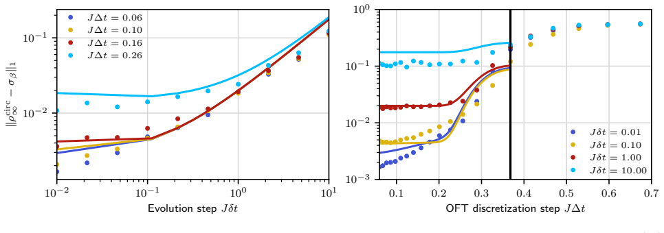
- Stochastic noise does not drive the state to the noise channel's fixed point: the bound $\|\tilde\rho_\infty-\sigma_\beta\|_1\le B\lambda/(1-(1-\lambda)e^{-\alpha})$ shows early-time errors are damped by the dissipative dynamics, and depolarizing circuit simulations confirm the predicted trade-off between algorithmic error and noise.
- Because $|\mathcal A|$ does not enter the circuit complexity of the Lindblad simulation, the steady-state accuracy can be improved by adding jump operators without increasing circuit depth, up to the limits of the jump operator model.
Reading between the lines
- Beyond the paper: the narrow frequency window $\Delta_{\rm RMT}=\Theta(1/\beta)$ is the empirical crux; measuring $|f(E,\nu)|^2$ for a chaotic local Hamiltonian across a range of $\beta$ would test whether the polynomial claims survive outside the single temperature $\beta=(2J)^{-1}$ used in the numerics.
- Beyond the paper: the observed steady-state error exponent ($\kappa\approx -0.2$ in $|\mathcal A|$ for chaotic points, versus $-1/2$ in the bound) hints that a fixed number of jump operators may keep $\|\rho_\infty-\sigma_\beta\|_1$ under control as $n$ grows; that would be stronger than Theorem 2 states.
- Beyond the paper: the coherent term $-i[H,\rho]$ drops out of the analytical gap calculation but visibly improves convergence in the numerics, suggesting the design space (filter shape, dissipation strength, partial coherent corrections) contains parameters that could further shorten mixing times.
- Beyond the paper: since the noise-resilience proof is for stochastic noise, applying randomized compiling to convert coherent hardware errors into stochastic channels would make the protocol's guarantees directly relevant to current devices.
Editorial analysis
A structured set of objections, weighed in public.
Referee Report
Summary. This paper proposes a Lindblad-engineering algorithm for preparing Gibbs states of non-commuting Hamiltonians. The Lindbladian (3) uses filtered operator-Fourier-transform jump operators built from local Pauli strings, with coherent part G = H, and the authors argue that under the eigenstate thermalization hypothesis (ETH) the ETH-averaged Lindbladian is approximately sigma_beta-detailed-balanced, has spectral gap Omega(1/(n beta^2)), and gives a mixing time O(n beta^2 (beta ||H||_infinity + log(1/epsilon))) with high probability (Thm. 2, Eqs. 17-18), provided the number of jump operators is poly(n, beta). The circuit implementation uses a single ancilla and a randomized selection of one jump operator per step, with Hamiltonian-simulation time Theta(beta t_mix^2 / epsilon sqrt(log(beta t_mix / epsilon))) (Thm. 1) and a detailed error budget (Prop. 1). A second contribution is a noise-resilience analysis (Thm. 3): for stochastic noise, early-time errors are damped by the contractive Lindblad dynamics. The claims are complemented by numerics for the mixed-field Ising model (n = 3,...,8, beta = (2J)^{-1}), including mixing-time and steady-state-distance scalings, and by full circuit simulations with depolarizing noise.
Significance. If the central theorem held as stated, the protocol would be a practically relevant simplification over CKG-style Gibbs samplers, and the single-ancilla randomized implementation with local Pauli jump operators is a genuine resource reduction. Strengths: the analytical derivation is elaborate and mostly self-contained; the error analysis of the circuit implementation (truncation, discretization, Trotter, dilation) is careful; the paper ships code and compiled circuits on GitHub; the numerical studies give falsifiable predictions (polynomial mixing in n in the chaotic regime, exponent kappa approx 1.4; |A|-dependence of the steady-state deviation with kappa approx -0.2); and the noise-resilience bound (Thm. 3) formalizes an effect usually only discussed informally. However, the headline quantitative claims are conditional on a structural assumption on the ETH off-diagonal function whose beta-dependence is neither standard nor tested, and the central theorem contains internal inconsistencies in the stated beta- and epsilon-scalings that must be fixed before the resource counts are reproducible.
major comments (4)
- [App. C.1, Assumption 1(b); Thm. 2] The polynomial-in-beta claim of Thm. 2 is conditional on Assumption 1(b), which is not a standard consequence of the ETH and is never probed in the numerics. The assumption is load-bearing: the conductance bounds in Eqs. (136)-(140) carry a factor e^{-beta Delta_RMT}, the gap bound (144) uses Delta_RMT^2 and the overlap Gamma, and the concentration estimates (162) and (171) use that f(nu) vanishes for |nu| > Delta_RMT. If the physical off-diagonal function for a chaotic Hamiltonian had support of width O(1) rather than Theta(1/beta), the same derivation would yield a gap Omega(e^{-O(beta)}/poly(n)) and a mixing time exponential in beta. The motivation in Eq. (107) only forces |f(nu)| to decay faster than e^{-beta nu/4} for large negative nu, which does not imply compact support of width 1/beta, so Assumption 1(b) is an added structural assumption, not a consequence of the ETH. All numerical studies fix beta = (2J)^{-1} (Sec. 5, App. D), so the assumed beta-dependence of Delta_RMT is never tested. I ask the authors to (i) state Thm. 2 in the abstract and introduction as conditional on Assumption 1(b), and (ii) provide a concrete test, e.g. extract |f(E,nu)| or its effective support width from eigenstate matrix elements of local observables in the chaotic lake of Eq. (30) at several beta, and/or scan t_mix as a function of beta at fixed n. These are well-posed and feasible checks; without them the claimed polynomial scaling in beta cannot be assessed.
- [Sec. 3.2, Eqs. (17)-(18); App. C.5, Eqs. (183), (192)-(194)] The quantitative statement of Thm. 2 has internal inconsistencies in the beta- and epsilon-scalings. Eq. (18) (and Thm. 2, Eq. (102)) quotes the steady-state error as O(epsilon + n beta^2 |A|^{-1/2} (beta ||H||_infinity + log(1/epsilon))), but the proof at Eq. (192) yields n beta^3 |A|^{-1/2} (...): gap^{-1} = O(n beta^2) from Eq. (146) times the channel distance O(beta/|A|^{1/2}) of Eq. (178). The sufficient number of jump operators is quoted as Omega(n^2 beta^6 ||H||^2_infinity / epsilon) in the main text after Eq. (18), as Omega(n^2 beta^8 ||H||^2_infinity / epsilon) in Eq. (194), as Omega(n^2 beta^6) in Eq. (183), and as Omega(n^2 beta^8) in the main text after Eq. (17); these statements differ by powers of beta. In addition, plugging |A| = Omega(n^2 beta^6 ||H||^2_infinity / epsilon) into Eq. (18) leaves a residual of order sqrt(epsilon) log(1/epsilon)/(beta ||H||_infinity), so the stated choice does not yield an epsilon-close steady state; the derivation implies |A| = Omega(n^2 beta^6 (beta ||H||_infinity + log(1/epsilon))^2 / epsilon^2) (with the beta-exponent shifted by two if one follows Eq. (192)). These mismatches should be reconciled so that the resource counts of Thm. 2 are reproducible; the qualitative polynomial dependence survives the correction.
- [Sec. 5.2, Eq. (31), Fig. 4] The numerical support for the claimed polynomial mixing-time scaling is weaker than the text suggests. The fits in Fig. 4 use six points (n = 3,...,8), report no error bars or bootstrap intervals, and the fitted exponents vary appreciably with |A| (e.g., for CH, kappa approx 1.09-1.26 for the mixing time and kappa approx -0.67 to -1.04 for the gap). Moreover, the mixing-time estimate (31) is computed from a single initial state, the maximally mixed state, whereas the mixing time in Eq. (7) is worst-case over all initial states; the text acknowledges this, but the plotted polynomial scaling is then an initial-state-dependent quantity, and for the REG point the trend is explicitly non-monotonic in n (Sec. 5.2, App. D.2.2). I recommend reporting bootstrap uncertainties on kappa and, at least for the chaotic point CH, the worst-case t_hat_mix over several random initial states (e.g., the Haar-random states already used in Fig. 15); the initial-state-independent spectral-gap data in the bottom row of Fig. 4 is the more robust witness of the polynomial trend.
- [Sec. 6.3, Eqs. (33)-(35), Fig. 6] The headline noise-resilience figures rest on an extrapolation whose hypotheses are only partially validated. The bound (35) requires the convergence inequality (33) to hold for all input states reachable under the noiseless dynamics (App. E.3), but B and alpha are fitted to a single initial state, rho(0) = I/2^n, for n = 3,...,8 (Sec. 6.3, App. E.4), and the fitted exponent alpha proportional to n^{-1.39} is quoted without uncertainty. Combined with the assumed gate model N_g = 50 n per step, this leads to the statement that at lambda_g = 10^{-8} Gibbs states of up to n = 100 qubits can be prepared with error approx 0.2. The text does flag the extrapolative nature of the estimate, but the phrasing under Fig. 6 reads as a concrete capability claim. I recommend reformulating that sentence as a heuristic extrapolation and, where feasible, testing the all-inputs condition on a few additional initial states at small n (the Haar-random states of Fig. 15 partially serve this purpose).
minor comments (4)
- [App. B.3, Eq. (85)] The statement that the number of Bohr frequencies satisfies |B_H| <= 4n is incorrect: for an n-qubit Hamiltonian the set of pairwise energy differences can have up to 4^n distinct elements. The Theta scaling in Eq. (85) only needs log|B_H| = O(n), so the asymptotic conclusion is unaffected, but the stated bound should be corrected.
- [Thm. 3 (App. E)] The theorem statement says 'with probability of no error incurring lambda', but the proof and Eq. (34) use lambda as the overall error probability; the two conventions should be aligned (error with probability lambda, no error with probability 1 - lambda).
- [Sec. 5.1] Typo: 'we ues a randomized simulation strategy' should read 'we use a randomized simulation strategy'.
- [App. D.3.3, Fig. 20] The statement that MCWF 'will likely require runtimes of around > 10^6 seconds' is an extrapolation beyond the plotted range of Fig. 20; stating the extrapolation method (e.g., a power-law fit in N_tra) would make the claim checkable.
Circularity Check
No significant circularity: the central ETH-based derivation is conditional on explicitly stated assumptions, and the numerical fits are labeled as such.
full rationale
I find no circularity in the paper's derivation chain. The main result, Theorem 2 (Eqs. 17-18), is a conditional derivation from an explicit ETH ansatz and additional stated assumptions. The ETH matrix-element form (Eq. 104), Assumption 1 on the off-diagonal function f(E,nu) (including the support width Delta_RMT = Theta(1/beta)), and Assumptions 2-3 on the density of states are all stated as inputs, not derived from the desired mixing-time result. The spectral-gap calculation (App. C.3) builds the classical Markov chain from the transition rates (Eq. 129), then bounds the conductance (Eqs. 136-143) and uses Cheeger's inequality to obtain Eq. (144); the final gap (Eq. 146) and mixing time (Eq. 182) follow from these ingredients plus the concentration bound (Eqs. 176-178). No equation is identified that is equivalent to the target result by construction. The concentration analysis invokes a matrix-concentration fact from prior work ([60], Fact D.1), but this is an auxiliary mathematical lemma with stated assumptions that do not include the target mixing-time result, so it does not constitute load-bearing self-citation. The numerical studies fit scaling exponents to simulated data and compare them with the analytic scaling; this is a consistency check, not a fitted quantity renamed as a prediction. In the noise analysis (Sec. 6.3) the paper explicitly says 'we fit B and alpha to numerical data' and stresses that the evaluation 'relies on extrapolation' of those fitted values to larger n, so it is a phenomenological evaluation rather than a derivation of the central claim. The most important caveat is correctly flagged by the paper itself in App. C.1: the polynomial-in-beta scaling relies on Assumption 1(b) (Delta_RMT = Theta(1/beta)), which is an unverified structural assumption about chaotic Hamiltonians, and the numerics fix beta = (2J)^-1 throughout so the beta-dependence is not empirically tested. This is a substantive correctness and assumption risk, but it is not circularity: the paper does not claim to derive Assumption 1(b), and the theorem is explicitly conditional on it.
Assumptions & free parameters
free parameters (4)
- Gaussian filter width Delta_E =
Delta_E = sqrt(2/beta) (Eq. 9, App. C.1)
- ETH off-diagonal parameters Delta_RMT and f0 =
Delta_RMT = Theta(1/beta), f0 constant (Assumption 1)
- Noise convergence fit parameters alpha and B =
alpha ~ O(n^{-1.39}), B ~ exp(-1.142 + 0.31 ln n) from Fig. 21 fits
- Circuit error fit coefficients alpha1..alpha4 =
Fitted in Eq. (37) to noiseless circuit simulation data (App. F)
assumptions (6)
- domain assumption ETH ansatz for local operators (Eq. 11 / Eq. 104): diagonal smooth function plus a random-matrix off-diagonal term with ER[R]=0, ER[|R|^2]=1
- ad hoc to paper Assumption 1(a,b): f(E,nu)=f(nu), flat on support [-Delta_RMT, Delta_RMT], with Delta_RMT = Theta(1/beta)
- domain assumption Assumption 2: bounded ratio of density of states, D(E)/D(E') <= R_D = Theta(1) for |E-E'| <= Delta_RMT
- domain assumption Assumption 3: the density of Gibbs states has bulk weight at least 1/2 and sufficiently fast tail decay
- standard math Uniqueness of the steady state when only multiples of the identity commute with H and the jump operators
- standard math Spectral gap to mixing time relation t_mix <= (1/Delta_L) log(2 ||rho_infinity^{-1/2}||_infty / epsilon) (Eq. 16)
Cite this review
Pith. "Pith review of Lindblad engineering for quantum Gibbs state preparation under the eigenstate thermalization hypothesis." pith.science (2026). https://pith.science/paper/P4YULEIO
@misc{pith2026241217706,
  author       = {Pith},
  title        = {Pith review of: Lindblad engineering for quantum Gibbs state preparation under the eigenstate thermalization hypothesis},
  year         = {2026},
  howpublished = {\url{https://pith.science/paper/P4YULEIO}},
  note         = {Machine review of arXiv:2412.17706}
}
read the original abstract
Building upon recent progress in Lindblad engineering for quantum Gibbs state preparation algorithms, we propose a simplified protocol that is shown to be efficient under the eigenstate thermalization hypothesis (ETH). The ETH reduces circuit overheads of the Lindblad simulation algorithm and ensures a fast convergence toward the target Gibbs state. Moreover, we show that the realized Lindblad dynamics exhibits an inherent resilience against stochastic noise, opening up the path to a first demonstration on quantum computers. We complement our claims with numerical studies of the algorithm's convergence in various regimes of the mixed-field Ising model. In line with our predictions, we observe a mixing time scaling polynomially with system size when the ETH is satisfied. In addition, we assess the impact of algorithmic and hardware-induced errors on the algorithm's performance by carrying out quantum circuit simulations of our Lindblad simulation protocol with a local depolarizing noise model. This work bridges the gap between recent theoretical advances in dissipative Gibbs state preparation algorithms and their eventual quantum hardware implementation.
Figures


Figures from the paper (19 more)




Reference graph
Works this paper leans on
-
[1]
Quantum Algorithms: A Survey of Applications and End-to-end Complexities
Alexander M. Dalzell, Sam McArdle, Mario Berta, Przemyslaw Bienias, Chi-Fang Chen, Andr´ as Gily´ en, Connor T. Hann, Michael J. Kastoryano, Emil T. Khabiboulline, Aleksander Kubica, Grant Salton, Samson Wang, and Fernando G. S. L. Brand˜ ao. “Quantum Algorithms: A Survey of Applications and End-to-end Complexities”. Cambridge University Press. Cambridge,...
arXiv 2025
-
[2]
Challenges and opportunities in quantum optimization
Amira Abbas, Andris Ambainis, Brandon Augustino, Andreas B¨ artschi, Harry Buhrman, Carleton Cof- frin, Giorgio Cortiana, Vedran Dunjko, Daniel J. Egger, Bruce G. Elmegreen, Nicola Franco, Filippo Fratini, Bryce Fuller, Julien Gacon, Constantin Gonciulea, Sander Gribling, Swati Gupta, Stuart Had- field, Raoul Heese, Gerhard Kircher, Thomas Kleinert, Thors...
2024
-
[3]
Problem of equilibration and the computation of correlation functions on a quantum computer
Barbara M. Terhal and David P. DiVincenzo. “Problem of equilibration and the computation of correlation functions on a quantum computer”. Phys. Rev. A 61, 022301 (2000)
2000
-
[4]
Sampling from the Thermal Quantum Gibbs State and Evaluating Partition Functions with a Quantum Computer
David Poulin and Pawel Wocjan. “Sampling from the Thermal Quantum Gibbs State and Evaluating Partition Functions with a Quantum Computer”. Phys. Rev. Lett. 103, 220502 (2009)
2009
-
[5]
Quantum Metropolis Sam- pling
K. Temme, T. J. Osborne, K. G. Vollbrecht, D. Poulin, and F. Verstraete. “Quantum Metropolis Sam- pling”. Nature 471, 87 (2011)
2011
-
[6]
Preparing thermal states of quantum systems by dimension reduction
Ersen Bilgin and Sergio Boixo. “Preparing thermal states of quantum systems by dimension reduction”. Phys. Rev. Lett. 105, 170405 (2010)
2010
-
[7]
A quantum–quantum Metropolis algorithm
Man-Hong Yung and Al´ an Aspuru-Guzik. “A quantum–quantum Metropolis algorithm”. Proc. Natl. Acad. Sci. U.S.A. 109, 754–759 (2012)
2012
-
[8]
Quantum Gibbs Samplers: The Commuting Case
Michael J. Kastoryano and Fernando G. S. L. Brand˜ ao. “Quantum Gibbs Samplers: The Commuting Case”. Commun. Math. Phys. 344, 915–957 (2016)
2016
Show all 115 references
-
[9]
Finite Correlation Length Implies Efficient Preparation of Quantum Thermal States
Fernando G. S. L. Brand˜ ao and Michael J. Kastoryano. “Finite Correlation Length Implies Efficient Preparation of Quantum Thermal States”. Commun. Math. Phys. 365, 1–16 (2019)
2019
-
[10]
Quantum algorithms for Gibbs sampling and hitting-time estimation
Anirban Narayan Chowdhury and Rolando D. Somma. “Quantum algorithms for Gibbs sampling and hitting-time estimation”. Quant. Inf. Comput. 17, 0041–0064 (2017)
2017
-
[11]
Determining eigenstates and thermal states on a quantum computer using quantum imaginary time evolution
Mario Motta, Chong Sun, Adrian Teck Keng Tan, Matthew J. O’ Rourke, Erika Ye, Austin J. Minnich, Fernando G. S. L. Brand˜ ao, and Garnet Kin-Lic Chan. “Determining eigenstates and thermal states on a quantum computer using quantum imaginary time evolution”. Nat. Phys. 16, 205–...
2019
-
[12]
Quantum singular value transformation and beyond: exponential improvements for quantum matrix arithmetics
Andr´ as Gily´ en, Yuan Su, Guang Hao Low, and Nathan Wiebe. “Quantum singular value transformation and beyond: exponential improvements for quantum matrix arithmetics”. In Proceedings of the 51st Annual ACM SIGACT Symposium on Theory of Computing. Pages 193–204. New York, NY,...
2019
-
[13]
Algorithms for Quantum Simulation at Finite Energies
Sirui Lu, Mari Carmen Ba˜ nuls, and J. Ignacio Cirac. “Algorithms for Quantum Simulation at Finite Energies”. PRX Quantum 2, 020321 (2021)
2021
-
[14]
Predicting Gibbs-State Expectation Values with Pure Thermal Shadows
Luuk Coopmans, Yuta Kikuchi, and Marcello Benedetti. “Predicting Gibbs-State Expectation Values with Pure Thermal Shadows”. PRX Quantum 4, 010305 (2023)
2023
-
[15]
Quantum algorithms from fluctuation theorems: Thermal-state preparation
Zoe Holmes, Gopikrishnan Muraleedharan, Rolando D. Somma, Yigit Subasi, and Burak S ¸ahino˘ glu. “Quantum algorithms from fluctuation theorems: Thermal-state preparation”. Quantum 6, 825 (2022)
2022
-
[16]
Dissipative Quantum Gibbs Sampling
Daniel Zhang, Jan Lukas Bosse, and Toby Cubitt. “Dissipative Quantum Gibbs Sampling” (2023). arXiv:2304.04526
2023 arXiv
-
[17]
Probing finite-temperature observables in quantum simulators of spin systems with short-time dynamics
Alexander Schuckert, Annabelle Bohrdt, Eleanor Crane, and Michael Knap. “Probing finite-temperature observables in quantum simulators of spin systems with short-time dynamics”. Phys. Rev. B 107, L140410 (2023)
2023
-
[18]
Robust Extraction of Thermal Observables from State Sampling and Real-Time Dynamics on Quantum Computers
Khaldoon Ghanem, Alexander Schuckert, and Henrik Dreyer. “Robust Extraction of Thermal Observables from State Sampling and Real-Time Dynamics on Quantum Computers”. Quantum 7, 1163 (2023)
2023
-
[19]
Measuring the Loschmidt Amplitude for Finite-Energy Properties of the Fermi-Hubbard Model on an Ion-Trap Quantum Computer
K´ evin H´ emery, Khaldoon Ghanem, Eleanor Crane, Sara L. Campbell, Joan M. Dreiling, Caroline Figgatt, Cameron Foltz, John P. Gaebler, Jacob Johansen, Michael Mills, Steven A. Moses, Juan M. Pino, Anthony Ransford, Mary Rowe, Peter Siegfried, Russell P. Stutz, Henrik Dreyer, ...
2024
-
[20]
Equation of State Calculations by Fast Computing Machines
Nicholas Metropolis, Arianna W. Rosenbluth, Marshall N. Rosenbluth, Augusta H. Teller, and Edward Teller. “Equation of State Calculations by Fast Computing Machines”. J. Chem. Phys. 21, 1087– 1092 (1953)
1953
-
[21]
Monte Carlo Sampling Methods Using Markov Chains and Their Applications
W. K. Hastings. “Monte Carlo Sampling Methods Using Markov Chains and Their Applications”. Biometrika 57, 97–109 (1970)
1970
-
[22]
Low-Depth Quantum Metropolis Algorithm
Jonathan E. Moussa. “Low-Depth Quantum Metropolis Algorithm” (2019). arXiv:1903.01451
2019 arXiv
-
[23]
Quantum Metropolis Sampling via Weak Measurement
Jiaqing Jiang and Sandy Irani. “Quantum Metropolis Sampling via Weak Measurement” (2024). arXiv:2406.16023
2024 arXiv
-
[24]
Universal quantum simulators
Seth Lloyd. “Universal quantum simulators”. Science 273, 1073–1078 (1996)
1996
-
[25]
On the Generators of Quantum Dynamical Semigroups
Goran Lindblad. “On the Generators of Quantum Dynamical Semigroups”. Commun. Math. Phys. 48, 119 (1976)
1976
-
[26]
Dissipative quantum church-turing theorem
M. Kliesch, T. Barthel, C. Gogolin, M. Kastoryano, and J. Eisert. “Dissipative quantum church-turing theorem”. Phys. Rev. Lett. 107, 120501 (2011)
2011
-
[27]
Efficient simulation of sparse Markovian quantum dynamics
Andrew M. Childs and Tongyang Li. “Efficient simulation of sparse Markovian quantum dynamics”. Quant. Inf. Comput. 17, 0901–0947 (2017)
2017
-
[28]
Efficient Quantum Algorithms for Simulating Lindblad Evolu- tion
Richard Cleve and Chunhao Wang. “Efficient Quantum Algorithms for Simulating Lindblad Evolu- tion” (2019). arXiv:1612.09512
2019 arXiv
-
[29]
Szegedy Walk Unitaries for Quantum Maps
Pawel Wocjan and Kristan Temme. “Szegedy Walk Unitaries for Quantum Maps”. Commun. Math. Phys. 402, 3201–3231 (2023)
2023
-
[30]
Preparing thermal states on noiseless and noisy programmable quantum processors
Oles Shtanko and Ramis Movassagh. “Preparing thermal states on noiseless and noisy programmable quantum processors” (2021). arXiv:2112.14688
2021 arXiv
-
[31]
Thermal State Preparation via Rounding Promises
Patrick Rall, Chunhao Wang, and Pawel Wocjan. “Thermal State Preparation via Rounding Promises”. Quantum 7, 1132 (2023)
2023
-
[32]
Quantum Thermal State Preparation
Chi-Fang Chen, Michael J. Kastoryano, Fernando G. S. L. Brand˜ ao, and Andr´ as Gily´ en. “Quantum Thermal State Preparation” (2023). arXiv:2303.18224
2023 arXiv
-
[33]
An efficient and exact noncommutative quantum Gibbs sampler
Chi-Fang Chen, Michael J. Kastoryano, and Andr´ as Gily´ en. “An efficient and exact noncommutative quantum Gibbs sampler” (2023). arXiv:2311.09207
2023
-
[34]
Single-ancilla ground state preparation via Lindbladians
Zhiyan Ding, Chi-Fang Chen, and Lin Lin. “Single-ancilla ground state preparation via Lindbladians”. Phys. Rev. Research 6, 033147 (2024)
2024
-
[35]
Efficient quantum Gibbs samplers with Kubo–Martin–Schwinger detailed balance condition
Zhiyan Ding, Bowen Li, and Lin Lin. “Efficient quantum Gibbs samplers with Kubo–Martin–Schwinger detailed balance condition”. Commun. Math. Phys. 406, 67 (2025). arXiv:2404.05998
2025 arXiv
-
[36]
Simulating Open Quantum Systems Using Hamiltonian Simula- tions
Zhiyan Ding, Xiantao Li, and Lin Lin. “Simulating Open Quantum Systems Using Hamiltonian Simula- tions”. PRX Quantum 5, 020332 (2024)
2024
-
[37]
Quantum generalizations of Glauber and Metropolis dynamics
Andr´ as Gily´ en, Chi-Fang Chen, Joao F. Doriguello, and Michael J. Kastoryano. “Quantum generalizations of Glauber and Metropolis dynamics” (2024). arXiv:2405.20322
2024
-
[38]
A Randomized Method for Simulating Lindblad Equations and Thermal State Preparation
Hongrui Chen, Bowen Li, Jianfeng Lu, and Lexing Ying. “A Randomized Method for Simulating Lindblad Equations and Thermal State Preparation” (2025). arXiv:2407.06594v3
2025
-
[39]
Quantum computation and quantum-state engineering driven by dissipation
Frank Verstraete, Michael M. Wolf, and J. Ignacio Cirac. “Quantum computation and quantum-state engineering driven by dissipation”. Nat. Phys. 5, 633–636 (2009)
2009
-
[40]
Preparation of entangled states by quantum Markov processes
B. Kraus, H. P. B¨ uchler, S. Diehl, A. Kantian, A. Micheli, and P. Zoller. “Preparation of entangled states by quantum Markov processes”. Phys. Rev. A 78, 042307 (2008)
2008
-
[41]
Engineered dissipation for quantum information science
Patrick M. Harrington, Erich J. Mueller, and Kater W. Murch. “Engineered dissipation for quantum information science”. Nat. Rev. Phys. 4, 660–671 (2022)
2022
-
[42]
Quantum Hamiltonian complexity in thermal equilibrium
Sergey Bravyi, Anirban Chowdhury, David Gosset, and Pawel Wocjan. “Quantum Hamiltonian complexity in thermal equilibrium”. Nat. Phys. 18, 1367–1370 (2022)
2022
-
[43]
Efficient thermalization and universal quantum computing with quantum Gibbs samplers
Cambyse Rouz´ e, Daniel Stilck Fran¸ ca, and´Alvaro M. Alhambra. “Efficient thermalization and universal quantum computing with quantum Gibbs samplers” (2024). arXiv:2403.12691
2024 arXiv
-
[44]
Quantum Computational Advantage with Constant-Temperature Gibbs Sampling
Thiago Bergamaschi, Chi-Fang Chen, and Yunchao Liu. “Quantum Computational Advantage with Constant-Temperature Gibbs Sampling”. In 2024 IEEE 65th Annual Symposium on Foundations of Computer Science (FOCS). Pages 1063–1085. (2024)
2024
-
[45]
Gibbs Sampling gives Quantum Advantage at Constant Tem- peratures with O(1)-Local Hamiltonians
Joel Rajakumar and James D. Watson. “Gibbs Sampling gives Quantum Advantage at Constant Tem- peratures with O(1)-Local Hamiltonians” (2024). arXiv:2408.01516
2024
-
[46]
Chaos and Quantum Thermalization
Mark Srednicki. “Chaos and Quantum Thermalization”. Phys. Rev. E 50, 888 (1994)
1994
-
[47]
Thermal fluctuations in quantized chaotic systems
Mark Srednicki. “Thermal fluctuations in quantized chaotic systems”. J. Phys. A: Math. Gen. 29, L75– L79 (1996). Accepted in Quantum 2025-08-20, click title to verify. Published under CC-BY 4.0. 59
1996
-
[48]
The approach to thermal equilibrium in quantized chaotic systems
Mark Srednicki. “The approach to thermal equilibrium in quantized chaotic systems”. J. Phys. A: Math. Gen. 32, 1163 (1999)
1999
-
[49]
From quantum chaos and eigenstate thermalization to statistical mechanics and thermodynamics
Luca D’Alessio, Yariv Kafri, Anatoli Polkovnikov, and Marcos Rigol. “From quantum chaos and eigenstate thermalization to statistical mechanics and thermodynamics”. Adv. Phys. 65, 239–362 (2016)
2016
-
[50]
Irreversible Thermodynamics for Quantum Systems Weakly Cou- pled to Thermal Reservoirs
Herbert Spohn and Joel L. Lebowitz. “Irreversible Thermodynamics for Quantum Systems Weakly Cou- pled to Thermal Reservoirs”. In Advances in Chemical Physics. Volume 38, pages 109–142. John Wiley & Sons, Ltd (1978)
1978
-
[51]
On the detailed balance condition for non-hamiltonian systems
Robert Alicki. “On the detailed balance condition for non-hamiltonian systems”. Rept. Math. Phys. 10, 249–258 (1976)
1976
-
[52]
Quantum detailed balance and KMS condition
Andrzej Kossakowski, Alberto Frigerio, Vittorio Gorini, and Maurizio Verri. “Quantum detailed balance and KMS condition”. Commun. Math. Phys. 57, 97–110 (1977)
1977
-
[53]
Gradient flow and entropy inequalities for quantum markov semigroups with detailed balance
Eric A. Carlen and Jan Maas. “Gradient flow and entropy inequalities for quantum markov semigroups with detailed balance”. Journal of Functional Analysis 273, 1810–1869 (2017)
2017
-
[54]
Generators of Detailed Balance Quantum Markov Semigroups
Franco Fagnola and Veronica Umanit` a. “Generators of Detailed Balance Quantum Markov Semigroups”. Infin. Dimens. Anal. Quantum Probab. Relat. Top. 10, 335–363 (2007)
2007
-
[55]
Generators of KMS Symmetric Markov Semigroups on B(h) Symmetry and Quantum Detailed Balance
Franco Fagnola and Veronica Umanit` a. “Generators of KMS Symmetric Markov Semigroups on B(h) Symmetry and Quantum Detailed Balance”. Commun. Math. Phys. 298, 523–547 (2010)
2010
-
[56]
The χ2-divergence and Mixing times of quantum Markov processes
K. Temme, M. J. Kastoryano, M. B. Ruskai, M. M. Wolf, and F. Verstraete. “The χ2-divergence and Mixing times of quantum Markov processes”. J. Math. Phys. 51, 122201 (2010)
2010
-
[57]
Quantum Channels & Operations Guided Tour
Michael M Wolf. “Quantum Channels & Operations Guided Tour”. Lecture notes. Niels-Bohr Institute, Copenhagen (2012). url: https://mediatum.ub.tum.de/doc/1701036/document.pdf
2012
-
[58]
Quantum simulation of Lindbladian dynamics via repeated interactions
Matthew Pocrnic, Dvira Segal, and Nathan Wiebe. “Quantum simulation of Lindbladian dynamics via repeated interactions”. J. Phys. A: Math. Theor. 58, 305302 (2025). arXiv:2312.05371
2025 arXiv
-
[59]
Mixing time of quantum Gibbs sampling for random sparse Hamiltonians
Akshar Ramkumar and Mehdi Soleimanifar. “Mixing time of quantum Gibbs sampling for random sparse Hamiltonians” (2024). arXiv:2411.04454
2024 arXiv
-
[60]
Fast Thermalization from the Eigenstate Thermalization Hypothesis
Chi-Fang Chen and Fernando G. S. L. Brand˜ ao. “Fast Thermalization from the Eigenstate Thermalization Hypothesis” (2021). arXiv:2112.07646
2021 arXiv
-
[61]
Optimal quantum algorithm for Gibbs state preparation
Cambyse Rouz´ e, Daniel Stilck Fran¸ ca, and´Alvaro M. Alhambra. “Optimal quantum algorithm for Gibbs state preparation” (2024). arXiv:2411.04885
2024
-
[62]
Relaxation times of dissipative many-body quantum systems
Marko Znidaric. “Relaxation times of dissipative many-body quantum systems”. Phys. Rev. E 92, 042143 (2015)
2015
-
[63]
Polynomial Time Quantum Gibbs Sampling for Fermi-Hubbard Model at any Temperature
ˇStˇ ep´ anˇSm ´ ıd, Richard Meister, Mario Berta, and Roberto Bondesan. “Polynomial Time Quantum Gibbs Sampling for Fermi-Hubbard Model at any Temperature” (2025) arXiv:2501.01412
2025
-
[64]
The Thermodynamic Cost of Ignorance: Thermal State Preparation with One Ancilla Qubit
Matthew Hagan and Nathan Wiebe. “The Thermodynamic Cost of Ignorance: Thermal State Preparation with One Ancilla Qubit” (2025) arXiv:2502.03410
2025 arXiv
-
[65]
Dissipative ground state preparation in ab initio electronic structure theory
Hao-En Li, Yongtao Zhan, and Lin Lin. “Dissipative ground state preparation in ab initio electronic structure theory” (2024). arXiv:2411.01470
2024
-
[66]
The quantum-jump approach to dissipative dynamics in quantum optics
M. B. Plenio and P. L. Knight. “The quantum-jump approach to dissipative dynamics in quantum optics”. Rev. Mod. Phys. 70, 101–144 (1998)
1998
-
[67]
Dephasing-induced diffusive transport in the anisotropic Heisenberg model
Marko Znidaric. “Dephasing-induced diffusive transport in the anisotropic Heisenberg model”. New J. Phys. 12, 043001 (2010)
2010
-
[68]
Corner-Space Renormalization Method for Driven-Dissipative Two-Dimensional Correlated Systems
S. Finazzi, A. Le Boit´ e, F. Storme, A. Baksic, and C. Ciuti. “Corner-Space Renormalization Method for Driven-Dissipative Two-Dimensional Correlated Systems”. Phys. Rev. Lett. 115, 080604 (2015)
2015
-
[69]
Adaptive variational low-rank dynamics for open quantum systems
Luca Gravina and Vincenzo Savona. “Adaptive variational low-rank dynamics for open quantum systems”. Phys. Rev. Research 6, 023072 (2024)
2024
-
[70]
Simulation methods for open quantum many-body systems
Hendrik Weimer, Augustine Kshetrimayum, and Rom´ an Or´ us. “Simulation methods for open quantum many-body systems”. Rev. Mod. Phys. 93, 015008 (2021)
2021
-
[71]
Large-scale stochastic simulation of open quantum systems
Aaron Sander, Maximilian Fr¨ ohlich, Martin Eigel, Jens Eisert, Patrick Gelß, Michael Hinterm¨ uller, Richard M. Milbradt, Robert Wille, and Christian B. Mendl. “Large-scale stochastic simulation of open quantum systems” (2025) arXiv:2501.17913
2025
-
[72]
Rapid quantum ground state preparation via dissipative dynamics
Yongtao Zhan, Zhiyan Ding, Jakob Huhn, Johnnie Gray, John Preskill, Garnet Kin-Lic Chan, and Lin Lin. “Rapid quantum ground state preparation via dissipative dynamics” (2025) arXiv:2503.15827
2025
-
[73]
Quantum chaos in the Bose-Hubbard model
A. R. Kolovsky and A. Buchleitner. “Quantum chaos in the Bose-Hubbard model”. EPL 68, 632 (2004)
2004
-
[74]
Multifractality of eigenfunctions in spin chains
Y. Y. Atas and E. Bogomolny. “Multifractality of eigenfunctions in spin chains”. Phys. Rev. E 86, 021104 (2012)
2012
-
[75]
Chaos and Ergodicity across the Energy Spectrum of Interacting Bosons
Lukas Pausch, Edoardo G. Carnio, Alberto Rodr ´ ıguez, and Andreas Buchleitner. “Chaos and Ergodicity across the Energy Spectrum of Interacting Bosons”. Phys. Rev. Lett. 126, 150601 (2021). Accepted in Quantum 2025-08-20, click title to verify. Published under CC-BY 4.0. 60
2021
-
[76]
Many-Body Interference at the Onset of Chaos
Eric Brunner, Lukas Pausch, Edoardo G. Carnio, Gabriel Dufour, Alberto Rodr ´ ıguez, and Andreas Buch- leitner. “Many-Body Interference at the Onset of Chaos”. Phys. Rev. Lett. 130, 080401 (2023)
2023
-
[77]
Ini- tialization of quantum simulators by sympathetic cooling
Meghana Raghunandan, Fabian Wolf, Christian Ospelkaus, Piet O. Schmidt, and Hendrik Weimer. “Ini- tialization of quantum simulators by sympathetic cooling”. Sci. Adv. 6, eaaw9268 (2020)
2020
-
[78]
Quantum digital cooling
Stefano Polla, Yaroslav Herasymenko, and Thomas E. O’Brien. “Quantum digital cooling”. Phys. Rev. A 104, 012414 (2021)
2021
-
[79]
Stable quantum-correlated many-body states through engineered dissipation
X. Mi et al. “Stable quantum-correlated many-body states through engineered dissipation”. Science 383, adh9932 (2024)
2024
-
[80]
Dissipative ground state preparation and the Dissipative Quantum Eigensolver
Toby S. Cubitt. “Dissipative ground state preparation and the Dissipative Quantum Eigensolver” (2023). arXiv:2303.11962
2023 arXiv
-
[81]
A noise-limiting quantum algorithm using mid-circuit measurements for dynamical correlations at infinite temperature
Etienne Granet and Henrik Dreyer. “A noise-limiting quantum algorithm using mid-circuit measurements for dynamical correlations at infinite temperature” (2024). arXiv:2401.02207
2024 arXiv
-
[82]
Accuracy Guarantees and Quantum Advantage in Analog Open Quantum Simulation with and without Noise
Vikram Kashyap, Georgios Styliaris, Sara Mouradian, J. Ignacio Cirac, and Rahul Trivedi. “Accuracy Guarantees and Quantum Advantage in Analog Open Quantum Simulation with and without Noise”. Phys. Rev. X 15, 021017 (2025)
2025
-
[83]
Quantum logarithmic Sobolev inequalities and rapid mixing
Michael J. Kastoryano and Kristan Temme. “Quantum logarithmic Sobolev inequalities and rapid mixing”. J. Math. Phys. 54, 052202 (2013)
2013
-
[84]
Random compiler for fast hamiltonian simulation
Earl Campbell. “Random compiler for fast hamiltonian simulation”. Phys. Rev. Lett. 123, 070503 (2019)
2019
-
[85]
Localization of interacting fermions at high temperature
Vadim Oganesyan and David A. Huse. “Localization of interacting fermions at high temperature”. Phys. Rev. B 75, 155111 (2007)
2007
-
[86]
Distribution of the Ratio of Consecutive Level Spacings in Random Matrix Ensembles
Y. Y. Atas, E. Bogomolny, O. Giraud, and G. Roux. “Distribution of the Ratio of Consecutive Level Spacings in Random Matrix Ensembles”. Phys. Rev. Lett. 110, 084101 (2013)
2013
-
[87]
Noise tailoring for scalable quantum computation via randomized compiling
Joel J. Wallman and Joseph Emerson. “Noise tailoring for scalable quantum computation via randomized compiling”. Phys. Rev. A 94, 052325 (2016)
2016
-
[88]
qujax: Simulating quantum circuits with JAX
Samuel Duffield, Gabriel Matos, and Melf Johannsen. “qujax: Simulating quantum circuits with JAX”. J. Open Source Softw. 8, 5504 (2023)
2023
-
[89]
JAX: composable transformations of Python+NumPy programs
James Bradbury, Roy Frostig, Peter Hawkins, Matthew James Johnson, Chris Leary, Dougal Maclau- rin, George Necula, Adam Paszke, Jake VanderPlas, Skye Wanderman-Milne, and Qiao Zhang. “JAX: composable transformations of Python+NumPy programs” (2018). Version 0.3.13. http://gith...
2018
-
[90]
t|ket⟩: a retargetable compiler for NISQ devices
Seyon Sivarajah, Silas Dilkes, Alexander Cowtan, Will Simmons, Alec Edgington, and Ross Duncan. “t|ket⟩: a retargetable compiler for NISQ devices”. Quantum Sci. Technol. 6, 014003 (2020)
2020
-
[91]
Robustness of adiabatic quantum computation
Andrew M. Childs, Edward Farhi, and John Preskill. “Robustness of adiabatic quantum computation”. Phys. Rev. A 65, 012322 (2001)
2001
-
[92]
Noise resistance of adiabatic quantum computation using random matrix theory
J´ er´ emie Roland and Nicolas J. Cerf. “Noise resistance of adiabatic quantum computation using random matrix theory”. Phys. Rev. A 71, 032330 (2005)
2005
-
[93]
Quantum advantage and stability to errors in analogue quantum simulators
Rahul Trivedi, Adrian Franco Rubio, and J. Ignacio Cirac. “Quantum advantage and stability to errors in analogue quantum simulators”. Nature Commun. 15, 6507 (2024)
2024
-
[94]
Effective quantum volume, fidelity and computational cost of noisy quantum processing experiments
K. Kechedzhi, S. V. Isakov, S. Mandr` a, B. Villalonga, X. Mi, S. Boixo, and V. Smelyanskiy. “Effective quantum volume, fidelity and computational cost of noisy quantum processing experiments”. Future Gener. Comput. Syst. 153, 431–441 (2024)
2024
-
[95]
The quantum adiabatic algorithm suppresses the proliferation of errors
Benjamin F. Schiffer, Adrian Franco Rubio, Rahul Trivedi, and J. Ignacio Cirac. “The quantum adiabatic algorithm suppresses the proliferation of errors” (2024). arXiv:2404.15397
2024 arXiv
-
[96]
Dilution of Error in Digital Hamiltonian Simulation
Etienne Granet and Henrik Dreyer. “Dilution of Error in Digital Hamiltonian Simulation”. PRX Quantum 6, 010333 (2025)
2025
-
[97]
Robustness of near-thermal dynamics on digital quantum computers
Eli Chertkov, Yi-Hsiang Chen, Michael Lubasch, David Hayes, and Michael Foss-Feig. “Robustness of near-thermal dynamics on digital quantum computers” (2024). arXiv:2410.10794
2024 arXiv
-
[98]
Randomized Compiling for Scalable Quantum Computing on a Noisy Superconducting Quantum Processor
Akel Hashim. “Randomized Compiling for Scalable Quantum Computing on a Noisy Superconducting Quantum Processor”. Phys. Rev. X 11, 041039 (2021)
2021
-
[99]
Learning quantum Hamiltonians at any temperature in polynomial time
Ainesh Bakshi, Allen Liu, Ankur Moitra, and Ewin Tang. “Learning quantum Hamiltonians at any temperature in polynomial time” (2023) arXiv:2310.02243
2023 arXiv
-
[100]
Bounds on chaos from the eigenstate thermalization hypothesis
Chaitanya Murthy and Mark Srednicki. “Bounds on chaos from the eigenstate thermalization hypothesis”. Phys. Rev. Lett. 123, 230606 (2019)
2019
-
[101]
Markovian master equations
E. B. Davies. “Markovian master equations”. Commun. Math. Phys. 39, 91–110 (1974)
1974
-
[102]
Markovian master equations. II
E. B. Davies. “Markovian master equations. II”. Math. Ann. 219, 147–158 (1976)
1976
-
[103]
New characteristic of quantum many-body chaotic systems
Anatoly Dymarsky and Hong Liu. “New characteristic of quantum many-body chaotic systems”. Phys. Rev. E 99, 010102 (2019). Accepted in Quantum 2025-08-20, click title to verify. Published under CC-BY 4.0. 61
2019
-
[104]
Entanglement and its relation to energy variance for local one-dimensional hamiltonians
Mari Carmen Ba˜ nuls, David A. Huse, and J. Ignacio Cirac. “Entanglement and its relation to energy variance for local one-dimensional hamiltonians”. Phys. Rev. B 101, 144305 (2020)
2020
-
[105]
Algorithms for quantum simulation at finite energies
Sirui Lu, Mari Carmen Ba˜ nuls, and J. Ignacio Cirac. “Algorithms for quantum simulation at finite energies”. PRX Quantum 2, 020321 (2021)
2021
-
[106]
Global characteristics of all eigenstates of local many- body Hamiltonians: participation ratio and entanglement entropy
W. Beugeling, A. Andreanov, and Masudul Haque. “Global characteristics of all eigenstates of local many- body Hamiltonians: participation ratio and entanglement entropy”. J. Stat. Mech. 2015, P02002 (2015)
2015
-
[107]
Quantum Ising model in transverse and longitudinal fields: chaotic wave functions
Y. Y. Atas and E. Bogomolny. “Quantum Ising model in transverse and longitudinal fields: chaotic wave functions”. J. Phys. A: Math. Theor. 50, 385102 (2017)
2017
-
[108]
Statistical properties of eigenstate amplitudes in complex quantum systems
Wouter Beugeling, Arnd B¨ acker, Roderich Moessner, and Masudul Haque. “Statistical properties of eigenstate amplitudes in complex quantum systems”. Phys. Rev. E 98, 022204 (2018)
2018
-
[109]
Ballistic Spreading of Entanglement in a Diffusive Nonintegrable System
Hyungwon Kim and David A. Huse. “Ballistic Spreading of Entanglement in a Diffusive Nonintegrable System”. Phys. Rev. Lett. 111, 127205 (2013)
2013
-
[110]
Mixing Time of Open Quantum Systems via Hypocoercivity
Di Fang, Jianfeng Lu, and Yu Tong. “Mixing Time of Open Quantum Systems via Hypocoercivity”. Phys. Rev. Lett. 134, 140405 (2025). arXiv:2404.11503
2025 arXiv
-
[111]
Wave-function approach to dissipative processes in quantum optics
Jean Dalibard, Yvan Castin, and Klaus Mølmer. “Wave-function approach to dissipative processes in quantum optics”. Phys. Rev. Lett. 68, 580–583 (1992)
1992
-
[112]
Monte Carlo simulation of the atomic master equation for spontaneous emission
R. Dum, P. Zoller, and H. Ritsch. “Monte Carlo simulation of the atomic master equation for spontaneous emission”. Phys. Rev. A 45, 4879–4887 (1992)
1992
-
[113]
Monte Carlo wave-function method in quantum optics
Klaus Mølmer, Yvan Castin, and Jean Dalibard. “Monte Carlo wave-function method in quantum optics”. J. Opt. Soc. Am. B 10, 524–538 (1993)
1993
-
[114]
QuTiP 2: A Python framework for the dynamics of open quantum systems
J. R. Johansson, P. D. Nation, and Franco Nori. “QuTiP 2: A Python framework for the dynamics of open quantum systems”. Comput. Phys. Commun. 184, 1234–1240 (2013)
2013
-
[115]
QuTiP 5: The Quantum Toolbox in Python
Neill Lambert, Eric Gigu` ere, Paul Menczel, Boxi Li, Patrick Hopf, Gerardo Su´ arez, Marc Gali, Jake Lishman, Rushiraj Gadhvi, Rochisha Agarwal, Asier Galicia, Nathan Shammah, Paul Nation, J. R. Johansson, Shahnawaz Ahmed, Simon Cross, Alexander Pitchford, and Franco Nori. “Q...
2024 arXiv
Reviewed August 11, 2026 · model on record in the stance chip above.
Discussion (0). Continue with ORCID to comment.