REVIEW 4 major objections 5 minor 6 references
A novel hybrid neural network of fluid-structure interaction prediction for two cylinders in tandem arrangement
T0 review · 4 major / 5 minor · reviewed 2026-08-16 · deepseek-v4-flash
Pith's one-line read A hybrid neural network predicts vortex-induced vibration of two tandem cylinders over 1000 times faster than CFD while tracking flow fields and structural motion.
desk verdict Useful FSI surrogate architecture, but the GIP displacement-feedback correction has a training/inference mismatch that undermines the headline accuracy; deserves peer review, not citation yet. read the letter →
The pith
A machine-rendered reading of the paper's core claim, the machinery that carries it, and where it could break.
The reading
What carries the argument
The load-bearing object is the USFNO-FConvLSTM flow-field model inside a recurrent FSI unit. The FNO part is a Fourier neural operator: a learnable integral operator that acts in frequency space using only the first $k_{\max}$ Fourier modes, which is what lets the network resolve the sharp zero-padded cylinder boundary as high-frequency content. The FConvLSTM part is the time-fusion module: it swaps the time and channel axes, runs a ConvLSTM over the $N$ historical steps, then linearly projects the fused features to one future state. The U-shaped tensor additions carry encoder features into the decoder to restore information lost in down-sampling. Around that core sit the MLP wall-shear model, which advances wall shear stress one step, the structural dynamics integrator, and the two coupling transfers: $F_b = F_{b-P} + F_{b-wall}$ from fluid to structure, and $U_F' = U_F \exp(y_{i-1})$ from structure to fluid. Together these form the USFNO-based FSI recurrent unit, and the whole network is a sequence of such units sharing hidden states.
What would settle it
Feed the trained network the true CFD displacement at each step instead of the network's own GIP-averaged displacement and compare flow-field errors. If the errors do not drop substantially, the displacement feedback is not carrying the boundary information; if they do, the closed-loop scheme depends on the readout being accurate. A second check: roll the network out for more than one vibration period and track the predicted cylinder boundary against the CFD mesh position; phase error growing without bound would falsify long-horizon reliability.
Extended reading notes
Core claim
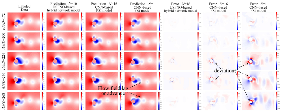
The central claim is that the proposed USFNO-based hybrid neural network can accurately and reliably predict the VIV evolution of two cylinders in tandem, including instantaneous flow-field states, wall shear stress, lift force, and structural displacement and velocity, at a fraction of the cost of CFD. The paper argues that this works because the flow-field model combines a Fourier neural operator, which captures the high-frequency gradient information at the moving cylinder edges, with a U-shaped encoder–decoder and a ConvLSTM variant that fuses $N$ historical time steps before projecting to one future state. The structural response is not learned: it is computed by fourth-order Runge–Kutta integration of the mass-damping-spring equation driven by forces integrated from the predicted pressure and wall-shear fields. Coupling is closed through force transfer from fluid to structure and through multiplicative displacement feedback $U_F' = U_F \exp(y_{i-1})$ from structure to fluid. The claim is comparative as well: with similar parameters, USFNO-FConvLSTM beats CNN- and Unet-based alternatives, and the multi-time-step FSI model beats its single-step CNN counterpart, especially for the interacting downstream cylinder.
Load-bearing premise
The load-bearing premise is that multiplying the low-dimensional flow features by $\exp(y_{i-1})$ and using a displacement that is itself partly read back from the predicted flow field faithfully encodes the moving boundary condition; if that feedback drifts, the closed-loop prediction will drift.
Editorial extensions
If this is right
- Multi-object VIV can be modeled without re-meshing: the next flow-field image is produced directly by the network, so the costly boundary-mesh update is bypassed.
- Wall shear stress is a necessary part of the force transfer at Re = 200; pressure-only integration visibly mis-fits the lift force, so neural FSI surrogates for low-Re flows should include it.
- Fusing about one vibration period of history (N = 16 of roughly 25 snapshots per cycle) improves accuracy; both shorter and longer histories degrade it, giving a design rule for sequence length.
- The same architecture transfers to an isolated cylinder, sustaining phase-coherent displacement and velocity prediction over long horizons, which supports generalization beyond the tandem configuration.
- For flow-field evolution the reported speedup is about 4020 times over the numerical solver, and for the full FSI loop more than 1000 times, which makes parameter sweeps and control studies practical.
Reading between the lines
- A testable extension would remove the exponential feedback and instead feed displacement as an extra input channel or additive term; if accuracy holds, the exponential form is not load-bearing, while if it fails, the moving-boundary encoding is doing more work than the flow-field network alone.
- Because errors accumulate with prediction horizon, re-initializing the flow-field state from a CFD snapshot or from a detected boundary position at regular intervals could stabilize very long rollouts; the paper does not test this.
- The gradient-based position readout (GIP) suggests the network localizes boundaries from image gradients; this could be extended to flexible structures by tracking a parameterized deformed boundary instead of a rigid translation.
- The same closed-loop architecture might apply to aeroelastic or marine-riser problems with multiple interacting bodies, but only if the training data cover the relevant reduced-velocity and spacing-ratio range; the paper explicitly lists multi-condition generalization as future work.
Signed reviews
Editorial analysis
A structured set of objections, weighed in public.
Referee Report
Summary. The manuscript proposes a hybrid neural-physics FSI solver for vortex-induced vibration of two elastically mounted cylinders in tandem and of an isolated cylinder at Re = 200. The fluid part is a novel USFNO-FConvLSTM network that predicts the next flow field from N historical flow fields and the current structural displacement; a separate MLP predicts wall shear stress; the structural response is advanced by a fourth-order Runge-Kutta solver. The two components exchange surface forces and displacement feedback (Eqs. 26-28). The authors report displacement MAE below 0.0006 m for the tandem case, pressure-field MAE/MRE of 0.0159 and 14.46% in the prediction phase, and prediction speeds over 1000x faster than CFD, with additional comparisons against CNN- and Unet-based baselines.
Significance. If the reported accuracy and speed hold under a properly specified training and evaluation protocol, the paper would make a useful contribution: a Fourier-operator-based recurrent surrogate for multi-body FSI and a modular coupling framework that goes beyond single-cylinder studies. The paper's strengths are its systematic study of fusion time steps (N = 16), its controlled architecture comparisons against CNN-FConvLSTM and Unet-FConvLSTM baselines, and the inclusion of both an isolated- and a tandem-cylinder case. These relative comparisons support the claim that the proposed flow-field architecture outperforms the authors' baselines. However, the absolute accuracy claims are not yet fully established because the closed-loop displacement feedback is trained with an oracle-selected correction scheme and the evaluation is limited to later time segments of the same simulation trajectories; no code or data are released, which further limits reproducibility.
major comments (4)
- [Sec. 4.4.2, Eq. (26)] The GIP displacement feedback is load-bearing, but the training procedure is not reproducible and is mismatched with inference. The text states that during training, after epoch 180, 'the better one between the computationally derived vibration displacement and that captured via gradient analysis is selected,' whereas in the predicting phase 'the average of the aforementioned two forms is adopted.' Since 'better' is evidently defined relative to the labeled displacement, the training feedback distribution is oracle-selected and differs from the averaged inference procedure. Because Eq. (26) injects y at time i-1 multiplicatively into the low-dimensional fluid features, the network is trained under more accurate boundary feedback than it receives in deployment, so the displacement MAE values in Tables 4-5 and the long roll-out accuracy shown in Figures 24-27 cannot be attributed to the published training procedure without an ablation. Please provide a full specification of the GIP algorithm (gradient computation, threshold, validation) and add an ablation comparing (a) ODE-only feedback, (b) average feedback from epoch 1, and (c) the oracle-selection schedule, reporting displacement and flow-field errors for each.
- [Sec. 4.1 and Sec. 4.4.2] The recurrent training procedure is under-specified, which matters because the model is autoregressive over the FSI loop. The manuscript does not state whether the USFNO-based FSI recurrent unit is trained with teacher forcing or closed-loop rollouts, how the loss is accumulated over the sequence, or how the epoch-180 GIP selection threshold was chosen. These details determine the distribution of the structural displacement seen by the flow-field network during training and directly influence the error-accumulation behavior reported in Figures 24-27. Please specify the exact training loop and report a sensitivity study over the switch epoch and over the choice of teacher forcing versus closed-loop training.
- [Sec. 4.4.1 and Sec. 4.4.2] The evaluation does not currently support the abstract's claim that the model can 'accurately and reliably predict' VIV evolution generically. For both the isolated-cylinder and tandem-cylinder cases, the prediction region is a later time segment of the same simulation trajectory used for training, so the test is in-sample temporal extrapolation rather than prediction for a new configuration. No experiment with different initial conditions, reduced velocity, or spacing ratio is reported, and the tandem case has only one trajectory. Please either add at least one unseen trajectory per case (e.g., different reduced velocity or initial disturbance) or explicitly restrict the claims to interpolation of the trained trajectory, which would be a more modest but defensible statement.
- [Sec. 2.1.1 and Eq. (1)] The wall shear stress module is described as a function of the previous wall shear stress alone, with no dependence on the predicted pressure field, the structural displacement, or the flow-field state. Yet the wall shear force from Eq. (28) is a component of the coupling force that drives the structural solver. As written, this module is an open-loop autoregressive model of the shear stress and does not receive the current boundary feedback used by the flow-field network. Please clarify whether the MLP is trained jointly with the flow-field model and whether the structural displacement or the predicted flow field enters its inputs; if the MLP is open-loop, the wall-shear force predictions in Figure 28 need to be re-evaluated in closed loop, and the 'fluid-structure interaction' characterization should be qualified.
minor comments (5)
- [Eq. (40)] The MRE formula is ambiguous as typeset: it should be written with explicit parentheses as the sum over i of absolute errors divided by the sum over i of absolute truth values, multiplied by 100 percent. Please rewrite the equation to avoid confusion between the summation over the error and the summation over the denominator.
- [Eqs. (8)-(9)] The discrete Fourier transform formulas contain garbled notation, including unclear exponential arguments and summation bounds. These should be rewritten with proper parentheses and explicit bounds for x1, x2, k1, and k2 so that the modes are unambiguous.
- [Sec. 4.3] The speedup claim of '4020 times faster' is reported without describing how the comparison was timed (GPU inference batching, number of CFD cores, warm-up, or memory transfer). Please provide the timing methodology and report both training time and inference time per rollout.
- [Data availability] The data availability statement says data are available from the corresponding author on request, but no code or pretrained models are mentioned. Given the many structural hyperparameters and the GIP threshold, releasing the implementation would substantially improve reproducibility.
- [General] The manuscript contains several typographical and notation inconsistencies, such as 'physis field features' in Section 2.1.2, 'FIS neural model' in Section 5, and the inconsistent use of the flow-field state notation; a careful proofreading pass is recommended.
Circularity Check
No significant circularity; the FSI model is a fitted surrogate evaluated on held-out time steps, and its predictions do not reduce to its inputs by construction.
full rationale
The paper's derivation chain is self-contained in the sense required by the circularity criteria. The flow-field model USFNO-FConvLSTM is trained on CFD-generated snapshots and then queried on later snapshots of the same simulation; this is a standard extrapolation-style test for a surrogate, not a situation where the predicted quantity is an input to its own derivation. The structural displacement is obtained by solving the discretized oscillator equation (Eq. 22-25) with forces integrated from predicted pressure and wall shear, which is a genuine forward coupling rather than a restatement of the target. The multiplicative feedback UF' = UF * exp(y_{i-1}) (Eq. 26) is an architecture choice, not an equation that presupposes the predicted future state. The GIP procedure described in Section 4.4.2 does introduce a train/test asymmetry: during training, after epoch 180, 'the better one between the computationally derived vibration displacement and that captured via gradient analysis is selected,' whereas in prediction 'the average of the aforementioned two forms is adopted as the temporal displacement.' This is a legitimate correctness and generalization concern, but it is not a circular reduction: the training-time selection is not the same operation as the deployment-time averaging, so the reported prediction errors are not equal to the training labels by construction. The paper also cites external prior work for FNO and ConvLSTM components rather than relying on a self-citation chain to justify its central claim. The numerical data are validated against published results in Tables 1-2, giving the fitted dataset independent support. Overall, no step in the paper's derivation chain reduces to its own inputs, so the appropriate circularity score is 0.
Assumptions & free parameters
free parameters (4)
- Fusion time steps N =
16
- Learning rate and decay =
0.001 (isolated), 0.0005 (tandem), decay base 0.977
- GIP selection threshold epoch =
180
- Network architecture dimensions =
not specified
assumptions (5)
- standard math Navier-Stokes equations govern the 2D laminar incompressible flow (Eq. 29).
- domain assumption VIV of the cylinders is modeled by a mass-damper-spring ODE with zero damping (Eq. 31-33).
- domain assumption The Fluent overset-mesh CFD results are accurate ground truth, validated against Zhao (2022) and Griffith et al. (2017) in Tables 1-2.
- domain assumption Nearest-neighbor interpolation to a 256x256 grid preserves the flow information needed for force integration.
- domain assumption Zero-filling the cylinder interior is an adequate representation for learning moving boundaries.
Cite this review
Pith. "Pith review of A novel hybrid neural network of fluid-structure interaction prediction for two cylinders in tandem arrangement." pith.science (2026). https://pith.science/paper/TTSWP4DZ
@misc{pith2026250414971,
  author       = {Pith},
  title        = {Pith review of: A novel hybrid neural network of fluid-structure interaction prediction for two cylinders in tandem arrangement},
  year         = {2026},
  howpublished = {\url{https://pith.science/paper/TTSWP4DZ}},
  note         = {Machine review of arXiv:2504.14971}
}
read the original abstract
Deep learning has shown promise in improving computing efficiency while ensuring modeling accuracy in fluid-structure interaction (FSI) analysis. However, its current capabilities are limited when it comes to constructing multi-object coupling systems with dynamic boundaries. To address such limitation, a novel FSI neural solver integrated by a fluid deep learning model with multi-time steps and a structural dynamic solver is proposed to accurately and reliably predict the vortex-induced vibration (VIV) evolution for two cylinders in tandem. This well-designed model in the form of end-to-end can precisely predict the instantaneous flow field state at the subsequent time by coupling the temporal flow fields of historical multi-time sequences and the current structural responses, moreover, derives the structural state at the next time. Furthermore, the novel fluid deep learning model consists of a wall shear model utilizing a multilayer perception network and flow field model with U-shaped architecture jointing the Fourier neural operator and modified convolution long-short term memory model. Both models effectively capture coupling transfer forces and predict instantaneous flow fields, with the latter demonstrating superior accuracy compared to Convolutional Neural Network- or Unet- based models with similar parameters. The prediction speed of the proposed models realizes an improvement of over 1000 times compared with the numerical simulation. Significantly, the proposed FSI neural model demonstrates exceptional capability in constructing the nonlinear complex multi- vibration systems and has substantial potential for advancing FSI modeling of flexible structures featuring pronounced nonlinear deformation boundaries.
Figures


Figures from the paper (26 more)




Reference graph
Works this paper leans on
-
[1]
Asefa, T., Kemblowski, M., McKee, M., & Khalil, A. (2006). Muli-time scale stream flow predictions: The support vector machines approach. Journal of hydrology, 318, 7-16. Beneddine, S., Yegavian, R., Sipp, D., & Leclaire, B. (2017). Unsteady flow dynamics reconstruction from mean flow and point sensors: an experimental study. Journal of Fluid Mechanics, 8...
arXiv 2006
-
[28]
Shirvani, A., Nili-Ahmadabadi, M., & Ha, M. Y . (2024). A deep learning-genetic algorithm approach for aerodynamic inverse design via optimization of pressure distribution. Computer methods in applied mechanics and engineering, 429, 117187. Srinivasan, P. A., Guastoni, L., Azizpour, H., Schlatter, P., & Vinuesa, R. (2019). Predictions of turbulent shear f...
work page 2024
-
[827]
Lv, Y . F., Sun, L. P., Bernitsas, M. M., & Sun, H. (2021). A comprehensive review of nonlinear oscillators in hydrokinetic energy harnessing using flow-induced vibrations. Renewable and Sustainable Energy Reviews, 150, 111388. Ma, A., Gibeau, B., & Ghaemi, S. (2020). Time-resolved topology of turbulent boundary layer separation over the training edge of ...
arXiv 2021
-
[893]
Rachit, G., & Rajeev, J. (2022). A hybrid partitioned deep learning methodology for moving interface and fluid-structure interaction. Computers and Fluids, 233, 105239. Ronneberger, O., Fischer, P., & Brox, T. (2015). U-net: Convolutional networks for biomedical image segmentation. In Medical image computing and computer-assisted intervention–MICCAI 2015:...
work page 2022
-
[1566]
He, P., & Qiao, R. (2011). A full-Eulerian solid level set method for simulation of fluid-structure interactions. Microfluidics and nanofluidics, 11, 557-567. He, X., Guo, Q. F., Xu, Y ., Feng, L. H., & Wang, J. J. (2022). Aerodynamics and fluid-structure 43 interaction on an airfoil with actively controlled flexible leeward surface. Journal of Fluid Mech...
work page 2011
-
[1780]
Q., Li, H., Chen, H., Wei, W., Wang, J
Hou, Y . Q., Li, H., Chen, H., Wei, W., Wang, J. Y ., & Huang, Y . C. (2022). A novel deep U-Net-LSTM framework for time-sequenced hydrodynamics prediction of the SUBOFF AFF-8. Engineering Applications of Computational Fluid Mechanics, 16(1), 630-645. Huang, G. J., Xia, Y . J., Dai, Y . T., Yang, C., & Wu, Y . (2021). Fluid-structure interaction in piezoe...
arXiv 2022
Reviewed August 16, 2026 · model on record in the stance chip above.
Discussion (0). Continue with ORCID to comment.